1. GAN
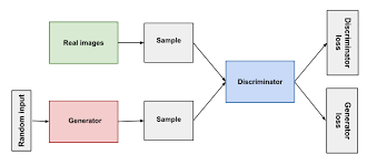
GAN(Generative Adversarial Network)은 생성자(Generator)와 판별자(Discriminator)라는 두 신경망이 경쟁하며 학습하는 구조이다.
생성자는 무작위 노이즈로부터 실제와 구분하기 어려운 데이터를 만들어내고,
판별자는 입력된 데이터가 진짜(실제 데이터)인지 가짜(생성자 출력)인지 구별하려 한다.
학습 과정에서 생성자는 판별자를 속이도록 점점 더 현실적인 데이터를 만들고,
판별자는 더 정밀하게 구분하도록 발전하여,
최종적으로는 매우 사실적인 이미지나 데이터 생성이 가능해진다.
2. GAN의 기본 아이디어
GAN(Generative Adversarial Network)은 두 개의 인공지능이 서로 경쟁하며 발전하는 구조이다.
- 생성자(Generator): “나는 진짜처럼 보이는 가짜 데이터를 만들 거야.”
- 판별자(Discriminator): “이 데이터가 진짜인지 가짜인지 내가 구분해 줄게.”
이 두 모델이 서로 경쟁하는데,
마치 위조지폐범(생성자)과 형사(판별자)의 대결과 비슷하다.
위조지폐범은 점점 더 정교하게 위조지폐를 만든다.
형사는 점점 더 눈썰미가 좋아져서 위조를 잘 잡아낸다.
이 과정을 반복하면, 결국 위조지폐는 진짜와 거의 구분이 안 갈 정도로 정교해진다.
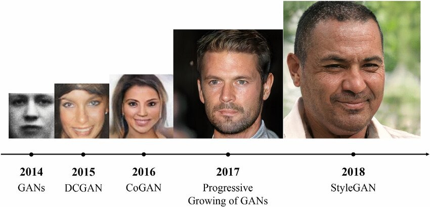
위 사진은 실제 인물이 아니라 GAN(Generative Adversarial Network)으로 생성된 가상 인물 이미지이다.
시간이 흐를수록 더 뚜렷하게 사람 이미지를 만들어내는 것이 신기하다.
3. GAN의 학습
4. DCGAN
DCGAN(Deep Convolutional GAN)은 전통적인 GAN 구조에 합성곱 신경망(CNN)을 적용하여 이미지 생성에 최적화된 모델이다.
생성자는 전치 합성곱(ConvTranspose2D)을 사용해 무작위 노이즈를 점점 업샘플링하며 이미지를 만들고, 판별자는 합성곱(Conv2D)으로 이미지를 다운샘플링하며 진짜·가짜를 구분한다.
또한 배치 정규화와 LeakyReLU/Tanh 활성화 등을 도입해 학습을 안정화하고, 풀링 연산 대신 스트라이드 합성곱을 사용하여 이미지의 공간적 패턴을 보존한다.
DCGAN은 보다 선명하고 사실적인 이미지를 생성할 수 있으며, 이후 다양한 GAN 변형 모델들의 기반이 되었다.
import random
import torch
import matplotlib.pyplot as plt
import numpy as np
import torchvision.utils as vutils
import torch.nn as nn
import torch.optim as optim
import matplotlib.animation as animation
from IPython.display import HTML
from torchvision.datasets import Food101
from torchvision.transforms import v2
manualSeed = 2025
random.seed(manualSeed) # Python random 시드 고정
torch.manual_seed(manualSeed) # PyTorch 시드 고정
torch.use_deterministic_algorithms(True) # 항상 같은 결과 보장 (재현성 확보)image_size = 64
dataset = Food101(
root=".", split="train", download=True, # Food101 학습용 데이터셋 다운로드
transform=v2.Compose([
v2.ToImage(), # 이미지를 Tensor 형태로 변환
v2.Resize((image_size, image_size), antialias=True), # 64x64 크기로 리사이즈
v2.ToDtype(torch.float32, scale=True), # float32로 변환 + [0,1] 스케일링
v2.Normalize((0.5, 0.5, 0.5), # 평균 0.5, 표준편차 0.5로 정규화
(0.5, 0.5, 0.5)), # 결과적으로 [-1,1] 범위로 맞춤
])
)workers = 2 # 데이터 로딩에 사용할 subprocess 개수
batch_size = 128 # 미니배치 크기
dataloader = torch.utils.data.DataLoader(
dataset,
batch_size=batch_size, # 한 번에 128개씩 로드
shuffle=True, # 매 epoch마다 데이터 순서 섞기
num_workers=workers # 병렬 로딩(2개 프로세스 사용)
)real_batch = next(iter(dataloader))
plt.figure(figsize=(8, 8))
plt.axis("off")
plt.title("Training Images")
plt.imshow(np.transpose(vutils.make_grid(real_batch[0][:64], padding=2, normalize=True),(1,2,0)))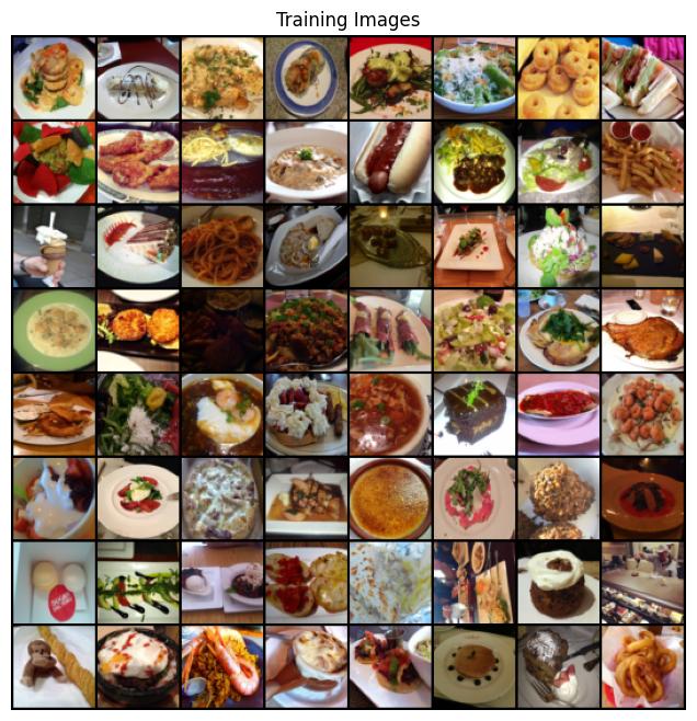
def weights_init(m):
    classname = m.__class__.__name__
    if classname.find('Conv') != -1:
        # Conv 계층: 평균 0, 표준편차 0.02로 초기화 (DCGAN 권장)
        nn.init.normal_(m.weight.data, 0.0, 0.02)
    elif classname.find('BatchNorm') != -1:
        # BatchNorm 계층: weight ~ N(1, 0.02), bias = 0
        nn.init.normal_(m.weight.data, 1.0, 0.02)
        nn.init.constant_(m.bias.data, 0)
device = torch.device("cuda:0" if torch.cuda.is_available() else "cpu")nc = 3 # 출력 이미지 채널 수 (RGB → 3)
ngf = 64 # Generator feature map 크기 (기본 채널 수)
nz = 100 # 잠재벡터(노이즈) 차원 (batch, nz, 1, 1)
# Generator (G)
class Generator(nn.Module):
def __init__(self):
super(Generator, self).__init__()
self.main = nn.Sequential(
# input is Z, going into a convolution
# 커널, 스트라이드, 패딩
nn.ConvTranspose2d( nz, ngf * 8, 4, 1, 0, bias=False),
nn.BatchNorm2d(ngf * 8),
nn.ReLU(True),
# state size. ``(ngf*8) x 4 x 4``
nn.ConvTranspose2d(ngf * 8, ngf * 4, 4, 2, 1, bias=False),
nn.BatchNorm2d(ngf * 4),
nn.ReLU(True),
# state size. ``(ngf*4) x 8 x 8``
nn.ConvTranspose2d( ngf * 4, ngf * 2, 4, 2, 1, bias=False),
nn.BatchNorm2d(ngf * 2),
nn.ReLU(True),
# state size. ``(ngf*2) x 16 x 16``
nn.ConvTranspose2d( ngf * 2, ngf, 4, 2, 1, bias=False),
nn.BatchNorm2d(ngf),
nn.ReLU(True),
# state size. ``(ngf) x 32 x 32``
nn.ConvTranspose2d( ngf, nc, 4, 2, 1, bias=False),
nn.Tanh()
# state size. ``(nc) x 64 x 64``
)
def forward(self, input):
return self.main(input)🟢 Generator (G) ― “이미지 만들기 공장”
Generator는 랜덤 노이즈 벡터를 받아서, 점점 해상도를 키우면서(업샘플링) 최종 이미지를 만들어낸다.
처음 입력은 (batch, 100, 1, 1) → 100차원짜리 랜덤 벡터
마지막 출력은 (batch, 3, 64, 64) → 64×64 RGB 이미지
단계별 설명
- ConvTranspose2d(nz → ngf*8)
- 100차원 노이즈 → (512, 4, 4) 이미지 블록
- ConvTranspose2d = 전치합성곱 (이미지를 키워주는 업샘플링 역할)
- ConvTranspose2d(ngf8 → ngf4)
- (512, 4×4) → (256, 8×8)
- 해상도가 커지면서 점점 "얼굴 윤곽" 같은 큰 구조를 그리기 시작
- ConvTranspose2d(ngf4 → ngf2)
- (256, 8×8) → (128, 16×16)
- 눈, 코, 입 같은 세부 패턴을 점점 더 잘 표현
- ConvTranspose2d(ngf*2 → ngf)
- (128, 16×16) → (64, 32×32)
- ConvTranspose2d(ngf → nc)
- (64, 32×32) → (3, 64×64)
- 최종 RGB 이미지 완성 (3은 채널 수: R,G,B)
- Tanh 활성화
- 픽셀 값을 [-1, 1] 범위로 맞춤 (학습 안정화)
ndf = 64 # Discriminator feature map 크기 (기본 채널 수)

# Discriminator (D)
class Discriminator(nn.Module):
    def __init__(self):
        super(Discriminator, self).__init__()
        self.main = nn.Sequential(
            # input is ``(nc) x 64 x 64``
            nn.Conv2d(nc, ndf, 4, 2, 1, bias=False),
            nn.LeakyReLU(0.2, inplace=True),
            # state size. ``(ndf) x 32 x 32``
            nn.Conv2d(ndf, ndf * 2, 4, 2, 1, bias=False),
            nn.BatchNorm2d(ndf * 2),
            nn.LeakyReLU(0.2, inplace=True),
            # state size. ``(ndf*2) x 16 x 16``
            nn.Conv2d(ndf * 2, ndf * 4, 4, 2, 1, bias=False),
            nn.BatchNorm2d(ndf * 4),
            nn.LeakyReLU(0.2, inplace=True),
            # state size. ``(ndf*4) x 8 x 8``
            nn.Conv2d(ndf * 4, ndf * 8, 4, 2, 1, bias=False),
            nn.BatchNorm2d(ndf * 8),
            nn.LeakyReLU(0.2, inplace=True),
            # state size. ``(ndf*8) x 4 x 4``
            nn.Conv2d(ndf * 8, 1, 4, 1, 0, bias=False),
            nn.Sigmoid()
        )

    def forward(self, input):
        return self.main(input)
🔴 Discriminator (D) ― “이미지 감별사”
Discriminator는 이미지를 입력받아 진짜/가짜 판별하는 역할을 한다.
입력은 (batch, 3, 64, 64) (RGB 이미지)
출력은 (batch, 1, 1, 1) → “진짜(1)냐? 가짜(0)냐?” 확률 값
단계별 설명
- Conv2d(nc → ndf)
- (3, 64×64) → (64, 32×32)
- 이미지를 절반으로 줄이면서 특징 뽑음
- Conv2d(ndf → ndf*2)
- (64, 32×32) → (128, 16×16)
- Conv2d(ndf2 → ndf4)
- (128, 16×16) → (256, 8×8)
- Conv2d(ndf4 → ndf8)
- (256, 8×8) → (512, 4×4)
- Conv2d(ndf*8 → 1)
- (512, 4×4) → (1, 1, 1)
- 진짜/가짜 여부를 출력
- Sigmoid 활성화
- 최종 출력값을 [0,1] 범위로 압축 → 확률처럼 해석
# 네트워크 생성 및 초기화
netG = Generator().to(device)   # Generator 생성
netD = Discriminator().to(device) # Discriminator 생성

netG.apply(weights_init)   # DCGAN 논문에서 제안한 방식으로 weight 초기화
netD.apply(weights_init)
Discriminator(
(main): Sequential(
(0): Conv2d(3, 64, kernel_size=(4, 4), stride=(2, 2), padding=(1, 1), bias=False)
(1): LeakyReLU(negative_slope=0.2, inplace=True)
(2): Conv2d(64, 128, kernel_size=(4, 4), stride=(2, 2), padding=(1, 1), bias=False)
(3): BatchNorm2d(128, eps=1e-05, momentum=0.1, affine=True, track_running_stats=True)
(4): LeakyReLU(negative_slope=0.2, inplace=True)
(5): Conv2d(128, 256, kernel_size=(4, 4), stride=(2, 2), padding=(1, 1), bias=False)
(6): BatchNorm2d(256, eps=1e-05, momentum=0.1, affine=True, track_running_stats=True)
(7): LeakyReLU(negative_slope=0.2, inplace=True)
(8): Conv2d(256, 512, kernel_size=(4, 4), stride=(2, 2), padding=(1, 1), bias=False)
(9): BatchNorm2d(512, eps=1e-05, momentum=0.1, affine=True, track_running_stats=True)
(10): LeakyReLU(negative_slope=0.2, inplace=True)
(11): Conv2d(512, 1, kernel_size=(4, 4), stride=(1, 1), bias=False)
(12): Sigmoid()
)
)criterion = nn.BCELoss() # 이진 크로스엔트로피(진짜/가짜 판별용 손실)
fixed_noise = torch.randn(64, nz, 1, 1, device=device) # 학습 과정 시각화용 고정 노이즈
real_label = 1.
fake_label = 0.
lr = 0.0002
beta1 = 0.5 # DCGAN 권장 베타(모멘텀 계열 안정화)
optimizerD = optim.Adam(netD.parameters(), lr=lr, betas=(beta1, 0.999))
optimizerG = optim.Adam(netG.parameters(), lr=lr, betas=(beta1, 0.999))img_list = [] # 생성 이미지 그리드 저장
G_losses = [] # G 손실 기록
D_losses = [] # D 손실 기록
iters = 0
num_epochs = 5
for epoch in range(num_epochs):
for i, data in enumerate(dataloader, 0):
###################
# (1) Discriminator 학습
netD.zero_grad()
real = data[0].to(device) # 진짜 이미지
b_size = real.size(0)
label = torch.full((b_size,), real_label, dtype=torch.float, device=device) # 1로 채움
output = netD(real).view(-1) # D(real)
errD_real = criterion(output, label) # 진짜에 대한 손실
errD_real.backward()
D_x = output.mean().item() # D(x)
noise = torch.randn(b_size, nz, 1, 1, device=device) # 가짜 만들 노이즈
fake = netG(noise) # G(z)
label.fill_(fake_label) # 0으로 채움(가짜 라벨)
output = netD(fake.detach()).view(-1) # D(G(z)) - detach로 G 고정
errD_fake = criterion(output, label) # 가짜에 대한 손실
errD_fake.backward()
D_G_z1 = output.mean().item() # 업데이트 전 D(G(z))
errD = errD_real + errD_fake # D 총 손실
optimizerD.step() # D 업데이트
###################
# (2) Generator 학습
netG.zero_grad()
label.fill_(real_label) # G는 D를 속여 1로 만들고 싶음
output = netD(fake).view(-1) # D(G(z)) (이번엔 detach 안 함)
errG = criterion(output, label) # G 손실
errG.backward()
D_G_z2 = output.mean().item() # 업데이트 후 D(G(z))
optimizerG.step() # G 업데이트
###################
# 로그/기록
if i % 50 == 0:
print(f"[{epoch}/{num_epochs}] [{i}/{len(dataloader)}]\tLoss_D: {errD.item():.4f}\tLoss_G: {errG.item():.4f}\tD(x): {D_x:.4f}\tD(G(z)): {D_G_z1:.4f} / {D_G_z2:.4f}")
G_losses.append(errG.item())
D_losses.append(errD.item())
# Loss_D : 낮을수록 잘 구분, Loss_G: 낮을수록 잘 속임,
# D(x): real 이미지를 얼마나 진짜로 보는지, D(G(z)): 업데이트 전 가짜 평균 / 업데이트 후 가짜 평균
if (iters % 500 == 0) or ((epoch == num_epochs-1) and (i == len(dataloader)-1)):
with torch.no_grad():
fake = netG(fixed_noise).detach().cpu() # 고정 노이즈로 스냅샷
img_list.append(vutils.make_grid(fake, padding=2, normalize=True))
iters += 1# 손실 곡선 시각화
plt.figure(figsize=(10,5))
plt.title("Generator and Discriminator Loss During Training")
plt.plot(G_losses,label="G")
plt.plot(D_losses,label="D")
plt.xlabel("iterations")
plt.ylabel("Loss")
plt.legend()
plt.show()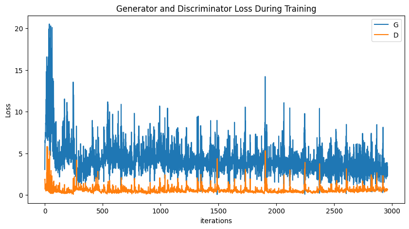
# 학습 과정에서 모은 img_list(그리드 이미지들)로 애니메이션 만들기
fig = plt.figure(figsize=(8,8))
plt.axis("off")
# img_list의 각 이미지 텐서를 (C,H,W)→(H,W,C)로 바꿔서 프레임 리스트 생성
ims = [[plt.imshow(np.transpose(i,(1,2,0)), animated=True)] for i in img_list]
# 1초 간격(interval=1000ms), 반복 전 1초 지연
ani = animation.ArtistAnimation(fig, ims, interval=1000, repeat_delay=1000, blit=True)

HTML(ani.to_jshtml())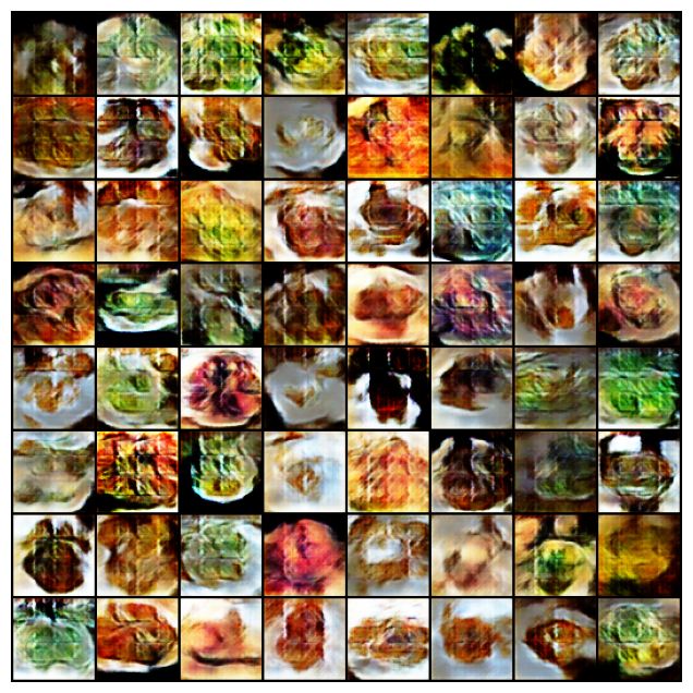
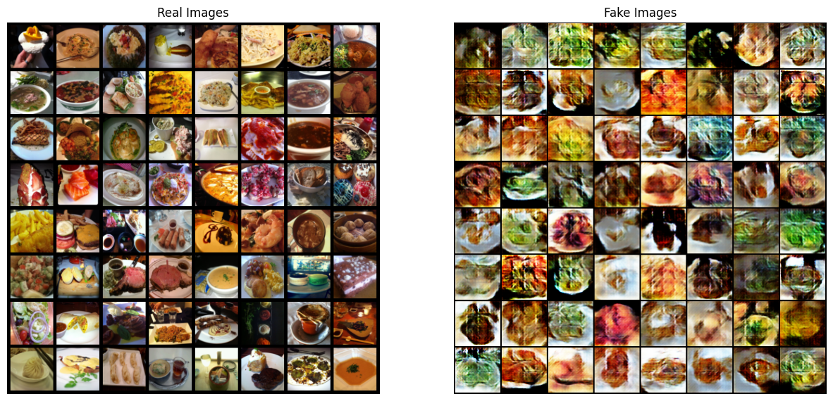
이렇게 가짜 이미지를 확인할 수 있었다.
# Real/Fake 이미지 그리드 나란히 시각화
real_batch = next(iter(dataloader)) # 배치 하나 꺼내기

plt.figure(figsize=(15,15))
plt.subplot(1,2,1)
plt.axis("off")
plt.title("Real Images")
# real_batch[0] = 이미지 텐서 (B,C,H,W)
# [:64] = 앞 64장 그리드로, normalize=True로 [-1,1]→[0,1] 스케일 복원
plt.imshow(np.transpose(vutils.make_grid(real_batch[0].to(device)[:64], padding=5, normalize=True).cpu(),(1,2,0)))

plt.subplot(1,2,2)
plt.axis("off")
plt.title("Fake Images")
# img_list[-1] = 마지막(가장 최근) 생성 결과 그리드
plt.imshow(np.transpose(img_list[-1],(1,2,0)))
plt.show()