1. 비지도 학습 (Unsupervised Learning)
비지도 학습은 정답(label)이 주어지지 않은 데이터를 기반으로 데이터의 구조, 패턴, 분포 등을 스스로 학습하는 방법이다.
입력 데이터만 가지고 유사한 데이터끼리 그룹화하거나(클러스터링), 데이터를 더 작은 차원으로 축소(차원 축소)하거나, 중요한 특징을 추출하는 것이 목표이다.
비지도 학습은 레이블링 비용이 많이 드는 현실적인 문제를 해결하고, 데이터에 대한 통찰을 얻는 데 유용하게 활용된다.
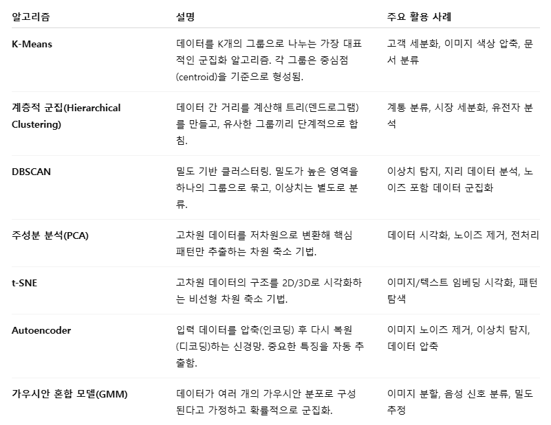
대표적인 비지도 학습 알고리즘
2. 클러스터링 (Clustering)
클러스터링은 정답(label) 없이 주어진 데이터를 유사한 특성을 가진 그룹(클러스터)으로 자동으로 나누는 방법이다.
데이터 간의 거리나 밀도, 연결 구조 등을 기준으로 군집을 형성한다.
대표적인 알고리즘 : K-means, DBSCAN, 계층적 군집(Hierarchical Clustering) 등
클러스터링은 고객 세분화, 문서 분류, 이미지 분할, 이상치 탐지 등 다양한 분야에 활용되며, 데이터를 시각적으로 이해하거나 패턴을 탐색할 때 매우 유용한 도구이다.
2-1. k-means
K-Means는 가장 널리 사용되는 클러스터링 알고리즘 중 하나로, 주어진 데이터를 K개의 클러스터로 나누는 비지도 학습 기법이다.
알고리즘은 먼저 무작위로 K개의 중심점을 선택한 후, 각 데이터를 가장 가까운 중심점에 할당하고, 각 클러스터의 중심을 다시 계산하는 과정을 반복한다.
이 과정을 통해 중심점이 더 이상 크게 이동하지 않을 때까지 수렴하며, 최종적으로 데이터는 유사한 특성을 가진 K개의 그룹으로 분류된다.
K-Means는 계산이 빠르고 구현이 간단하다.
하지만, 클러스터 수(K)를 사전에 정해야 하며, 복잡한 형태나 밀도 차이가 큰 데이터에는 적합하지 않을 수 있다.
- "몇 개의 그룹으로 나눌 것인지" 결정한다. ex) K=2, 2개의 클러스터로 나눔
- 데이터 공간에서 K개의 중심점을 무작위로 뽑는다. 이 중심점은 클러스터의 대표값 역할을 한다.
- 모든 데이터 포인트에 대해 각 중심점과의 거리를 계산하고, 가장 가까운 중심점에 소속되도록 할당한다. → K개의 그룹이 만들어짐
- 각 클러스터에 속한 데이터들의 평균값을 계산해서 중심점을 새로 위치시킨다. → 중심점이 데이터 분포의 중심으로 이동한다.
- 데이터의 소속 그룹이 바뀌지 않을 때까지, 또는 중심점의 이동이 거의 없을 때까지 반복한다. → 수렴(convergence)
import pandas as pd
import seaborn as sns
from sklearn.datasets import make_blobs # 가짜 데이터(군집용) 생성 함수
from sklearn.cluster import KMeans  # KMeans 클러스터링 알고리즘
샘플 데이터 생성
# - n_samples=100 → 총 100개 점 생성
# - centers=3 → 3개의 중심(클러스터)을 기준으로 점들을 분포시킴
# - random_state=2025 → 난수 고정 (재현성 확보)

X, y = make_blobs(n_samples=100, centers=3, random_state=2025)
print(X) # X: 100개의 (x, y) 좌표 데이터 (shape: 100 x 2)y # y: 각 점이 속한 실제 클러스터 레이블 (0,1,2 중 하나)출력 예시 → 0,1,2 라벨로 각 점의 군집이 미리 지정되어 있음 (정답 라벨)
array([1, 2, 0, 0, 2, 1, 2, 0, 2, 1, 1, 0, 0, 1, 1, 0, 0, 1, 1, 2, 0, 1,
       2, 0, 1, 0, 0, 1, 1, 2, 2, 0, 0, 1, 1, 1, 0, 2, 0, 0, 0, 1, 0, 2,
       1, 2, 1, 1, 2, 2, 0, 1, 2, 2, 2, 2, 2, 0, 2, 0, 1, 1, 1, 1, 2, 0,
       1, 1, 0, 0, 2, 0, 2, 1, 2, 0, 0, 1, 2, 2, 2, 2, 1, 2, 2, 1, 0, 2,
       0, 1, 0, 0, 0, 2, 1, 1, 2, 0, 0, 2])
DataFrame 변환
# X는 numpy 배열 형태라 다루기 불편할 수 있음
# → Pandas DataFrame으로 변환하여 컬럼 단위로 쉽게 다룰 수 있음

X = pd.DataFrame(X)
X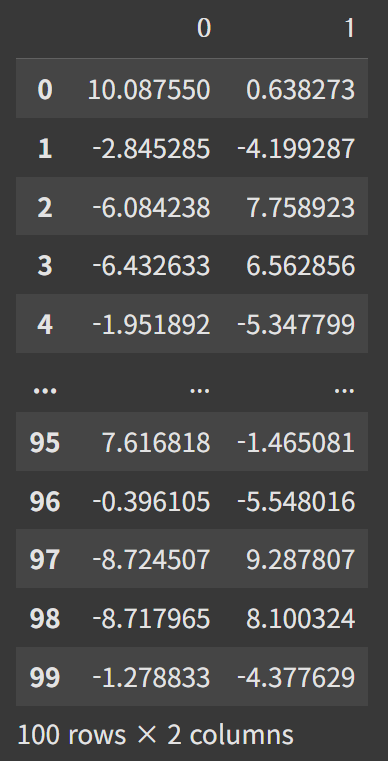
원본 데이터 시각화
# - x축: X의 첫 번째 컬럼 (0번)
# - y축: X의 두 번째 컬럼 (1번)
# - 색상(hue): 실제 레이블(y)

sns.scatterplot(x=X[0], y=X[1], hue=y)
KMeans 모델 생성 및 학습
# - n_clusters=3 → 3개의 클러스터로 데이터 분할

km = KMeans(n_clusters=3)
# X 데이터로 모델 학습 (중심점 찾기)
km.fit(X)
# 예측 (클러스터 할당)
# - 학습된 클러스터 중심을 기준으로 각 점이 어디 속할지 예측
pred = km.predict(X)
KMeans 예측 결과 시각화
# - 실제 레이블(y) 대신 예측된 클러스터 번호(pred)를 색상(hue)으로 사용

sns.scatterplot(x=X[0], y=X[1], hue=pred)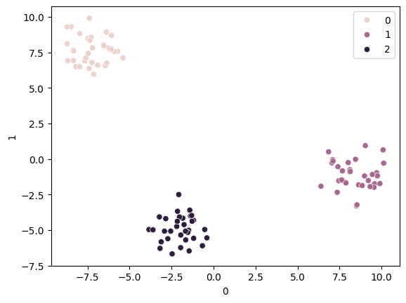
km = KMeans(n_clusters=5)
km.fit(X)
pred = km.predict(X)
sns.scatterplot(x=X[0], y=X[1], hue=pred)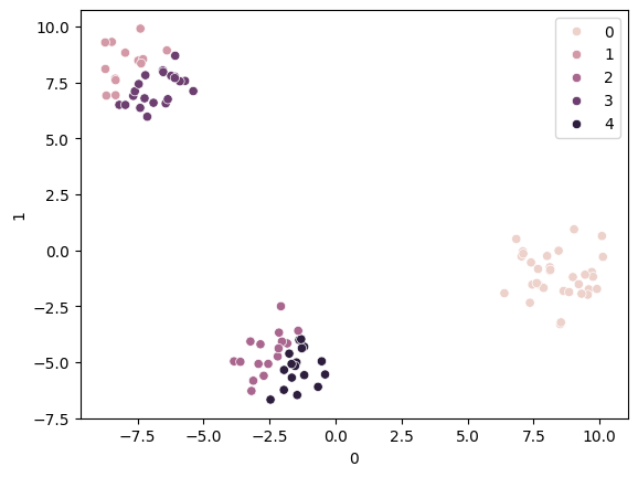
'''
inertia_는 각 데이터 포인트와 자신이 속한 클러스터 중심점(centroid)
사이의 거리 제곱합(Sum of Squared Distances)입니다.
즉, 클러스터 내에서 데이터들이 중심점에 얼마나 가까이 모여 있는지를
수치로 나타냅니다.
'''
km.inertia_ # (클러스터 내 거리 제곱합)140.22652512243334# inertia 값을 저장할 리스트
inertia_list = []
# 클러스터 개수를 2~10까지 바꿔가며 KMeans 학습
for i in range(2, 11):
km = KMeans(n_clusters=i) # i개의 클러스터
km.fit(X) # 모델 학습
inertia_list.append(km.inertia_) # inertia 저장# inertia 값 출력
inertia_list[2202.099288979431,
178.3026813479228,
149.2341882048366,
137.61757173359808,
107.83047351836134,
90.81946104617326,
81.1567801922611,
67.89497828315466,
59.77392846231832]inertia 값 시각화 (엘보우 기법)
# - x축: 클러스터 개수
# - y축: inertia (작을수록 데이터가 중심에 잘 모여 있음)

sns.lineplot(x=range(2, 11), y=inertia_list)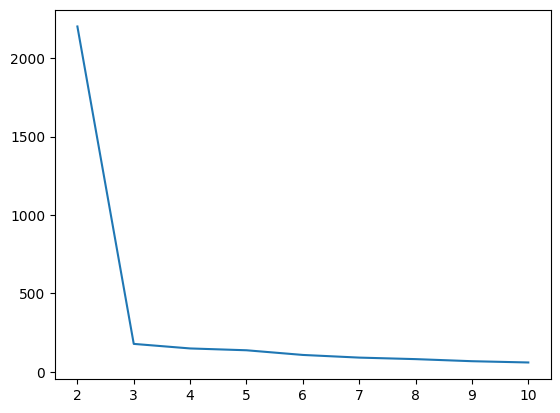
엘보우(Elbow) 메서드
클러스터링에서 최적의 클러스터 수(K)를 찾기 위한 직관적인 방법이다.
이 방법은 K를 1부터 점차 늘려가며 각 K 값에 대한 클러스터 내 거리 제곱합(inertia_)을 계산하고, 이를 그래프로 나타낸다.
K가 증가할수록 inertia 값은 감소하지만, 어느 순간부터 감소 속도가 완만해지는데, 이때 그래프가 팔꿈치(elbow)처럼 꺾이는 지점을 최적의 K로 선택한다.
이 지점은 모델이 충분히 군집을 잘 나누되, 과도하게 세분화하지 않는 균형점으로 간주된다.
2-2. 계층적 군집 (Hierarchical Clustering)
계층적 군집은 데이터 간의 유사도를 기준으로 계층 구조의 트리(dendrogram)를 생성하며, 이를 통해 데이터를 점진적으로 군집화하는 비지도 학습 기법이다.
크게 병합형(agglomerative)과 분할형(divisive)으로 나뉘며,
병합형은 각 데이터를 개별 클러스터로 시작해 가장 유사한 것부터 합쳐가고,
분할형은 전체 데이터를 하나의 클러스터로 시작해 점차 분리해 나간다.
이 알고리즘은 클러스터 수를 사전에 정하지 않아도 되며, 덴드로그램을 통해 적절한 군집 수를 시각적으로 판단할 수 있는 장점이 있다.
하지만 계산 복잡도가 높아 대용량 데이터에는 비효율적일 수 있다.
- 병합형 계층적 군집의 예
- 처음에는 N개의 데이터가 있으면 N개의 클러스터로 간주한다.
- 데이터 간 거리(혹은 클러스터 간 거리)를 계산해서 가장 가까운 두 개를 선택해 합친다.
- 두 클러스터가 합쳐졌기 때문에, 새로 생긴 클러스터와 나머지 클러스터들과의 거리를 다시 계산한다.
Step 2로 돌아가 계속 합친다.- 모든 데이터가 하나의 클러스터가 될 때까지 반복
import torch
import numpy as np
from torchvision.transforms import v2
from torchvision.datasets import MNIST
Transform 정의
# ToImage(): PIL.Image나 NumPy 배열 → PyTorch 텐서 (C, H, W) 구조로 변환
#   - PyTorch의 기본 이미지 텐서는 (채널, 높이, 너비) = (C, H, W)
#   - 일반 NumPy/OpenCV는 (H, W, C)이므로 순서를 맞춰줌
#   - dtype도 PyTorch 텐서에 맞게 변환 (예: uint8 → torch.float32)
#
# Lambda(torch.flatten): 2D 이미지를 1D 벡터로 펼치기
#   - MNIST 이미지는 (1, 28, 28) → flatten → (784,)
#   - 즉, 28x28 픽셀을 길이 784짜리 벡터로 만듦

transforms = v2.Compose([
    v2.ToImage(),
    v2.Lambda(torch.flatten),
])

# MNIST 데이터셋 로드
# train=False → 테스트 세트 (10000개 샘플)
# download=True → 데이터가 없으면 자동 다운로드
# transform=transforms → 위에서 정의한 변환 적용

flatten_mnist = MNIST(".", train=False, download=True, transform=transforms)
len(flatten_mnist) # 10000무작위로 30개 샘플 선택
np.random.seed(2025) # 시드 고정 (재현성)
mnist_indices = np.random.choice(len(flatten_mnist), 30, replace=False)
mnist_indices # (랜덤으로 뽑힌 30개 인덱스)
array([6448, 3544, 3904, 9739, 8295, 3600, 1457, 6938, 984, 9586, 9652,
6662, 2470, 6386, 6193, 2565, 1394, 5215, 592, 6296, 5188, 3458,
3048, 7557, 3524, 1684, 8461, 8814, 5643, 9259])실제 이미지 & 레이블 추출
# flatten_mnist[idx]는 (이미지 텐서, 라벨) 튜플 반환
# 이미지 텐서를 numpy 배열로 변환하여 리스트로 모음
flatten_X = np.array([flatten_mnist[idx][0].numpy() for idx in mnist_indices])

# 각 이미지에 대응되는 레이블(y) 추출
flatten_y = np.array([flatten_mnist[idx][1] for idx in mnist_indices])
flatten_X # → shape: (30, 784) (30개 샘플, 각각 784차원 벡터)
flatten_y array([4, 4, 2, 0, 2, 2, 0, 1, 1, 7, 7, 7, 8, 5, 2, 7, 8, 3, 0, 8, 8, 0,
2, 9, 6, 5, 3, 6, 2, 2])from sklearn.cluster import AgglomerativeClustering
from matplotlib import pyplot as plt
from scipy.cluster.hierarchy import dendrogramAgglomerative (병합) 클러스터링
# 샘플을 하나씩 클러스터로 시작해, 가장 가까운 두 클러스터를 반복적으로 병합
# compute_distances=True, model.distances_ 에 병합 거리를 저장
# n_clusters=2: 최종적으로 2개 클러스터가 되면 멈춤
# metric='euclidean': 샘플 간 거리는 유클리드 계산
# 속성
# model.labels_: 각 샘플의 군집 라벨
# model.children_: 병합된 두 클러스터의 인덱스 기록
# model.distances_: 병합 시의 거리
# model.n_clusters_: 최종 군집 개수

model = AgglomerativeClustering(compute_distances=True)

# 클러스터 학습 (트리 구조 생성)
model = model.fit(flatten_X)
덴드로그램 유틸 함수
def plot_dendrogram(model, labels):

    """
    sklearn의 AgglomerativeClustering 결과를
    scipy dendrogram()이 요구하는 linkage_matrix 형식으로 변환해 그린다.

    매 병합 단계 i에 대해:
      - model.children_[i] : 병합된 두 '노드'의 인덱스 (샘플(<n_samples) or 내부노드(>=n_samples))
      - model.distances_[i]: 그 두 노드의 거리
      - counts[i]          : 병합된 서브트리에 포함된 leaf(원 샘플) 개수 (가지 수)
    """
    # 병합 단계 수 = n_samples - 1
    counts = np.zeros(model.children_.shape[0])
    n_samples = len(model.labels_)

    for i, merge in enumerate(model.children_):
        current_count = 0
        for child_idx in merge:
            if child_idx < n_samples:
            	# child_idx가 원 샘플(leaf)이면 1개 추가
                current_count += 1  # leaf node
            else:
            	# 내부 노드면, 그 노드에 속한 leaf 개수를 더함
                current_count += counts[child_idx - n_samples]
        counts[i] = current_count

	# scipy.dendrogram 이 요구하는 linkage_matrix 구성:
    #   [ [child1, child2, distance, leaf_count], ... ]
    linkage_matrix = np.column_stack(
        [model.children_, model.distances_, counts]
    ).astype(float)

    dendrogram(linkage_matrix, labels=labels, truncate_mode=None, distance_sort='descending')
plot_dendrogram 함수 흐름
1. 모델이 주는 정보
예를 들어 데이터가 5개 있다고 해보자. (샘플 개수 = 5)
model.children_ = [
    [0, 1],  # 샘플 0과 1이 합쳐짐
    [2, 5],  # 샘플 2와 (0+1) 군집이 합쳐짐 → 새 index 5
    [3, 4],  # 샘플 3과 4가 합쳐짐
    [6, 7]   # (2+(0,1)) 군집과 (3,4) 군집이 합쳐짐
]

model.distances_ = [
    0.5,  # 0-1 거리
    1.2,  # 2-(0,1) 거리
    0.8,  # 3-4 거리
    2.5   # 전체 합쳐지는 거리
]
여기서 5, 6, 7 같은 숫자는 원래 데이터가 아니라,
앞에서 합쳐진 클러스터를 새로 번호 붙여서 나타낸 것이다.
(n_samples=5일 때 새 번호는 5부터 시작)
2. counts 계산
counts = np.zeros(model.children_.shape[0])counts 배열은 각 병합에서 해당 클러스터에 포함된 원래 데이터 개수를 저장한다.
#ex)

[0, 1] → 리프(원래 데이터) 2개 → count = 2

[2, 5] → 1개(리프 2) + 2개(클러스터 5) → count = 3

[3, 4] → 리프 2개 → count = 2

[6, 7] → 3개 + 2개 → count = 5
3. linkage_matrix 만들기
linkage_matrix = np.column_stack(
    [model.children_, model.distances_, counts]
)
SciPy의 dendrogram() 함수는 반드시 linkage_matrix를 입력으로 받아야 한다.
여기서 각 행의 의미
[왼쪽 index, 오른쪽 index, 두 군집 사이 거리, 병합된 샘플 개수]4. 덴드로그램 그리기
dendrogram(linkage_matrix, labels=labels, distance_sort='descending')- 리프 노드(맨 아래) → 원래 데이터
- 위로 올라가면서 선이 합쳐지는 부분 → 군집이 병합되는 과정
- 선의 높이 → model.distances_ (군집 간 거리)
덴드로그램 그리기
plt.figure(figsize=(20, 8))
plt.title("MNIST Clustering Dendrogram")
plot_dendrogram(model, flatten_y) # flatten_y: 각 샘플의 실제 숫자 라벨(0~9)
plt.show()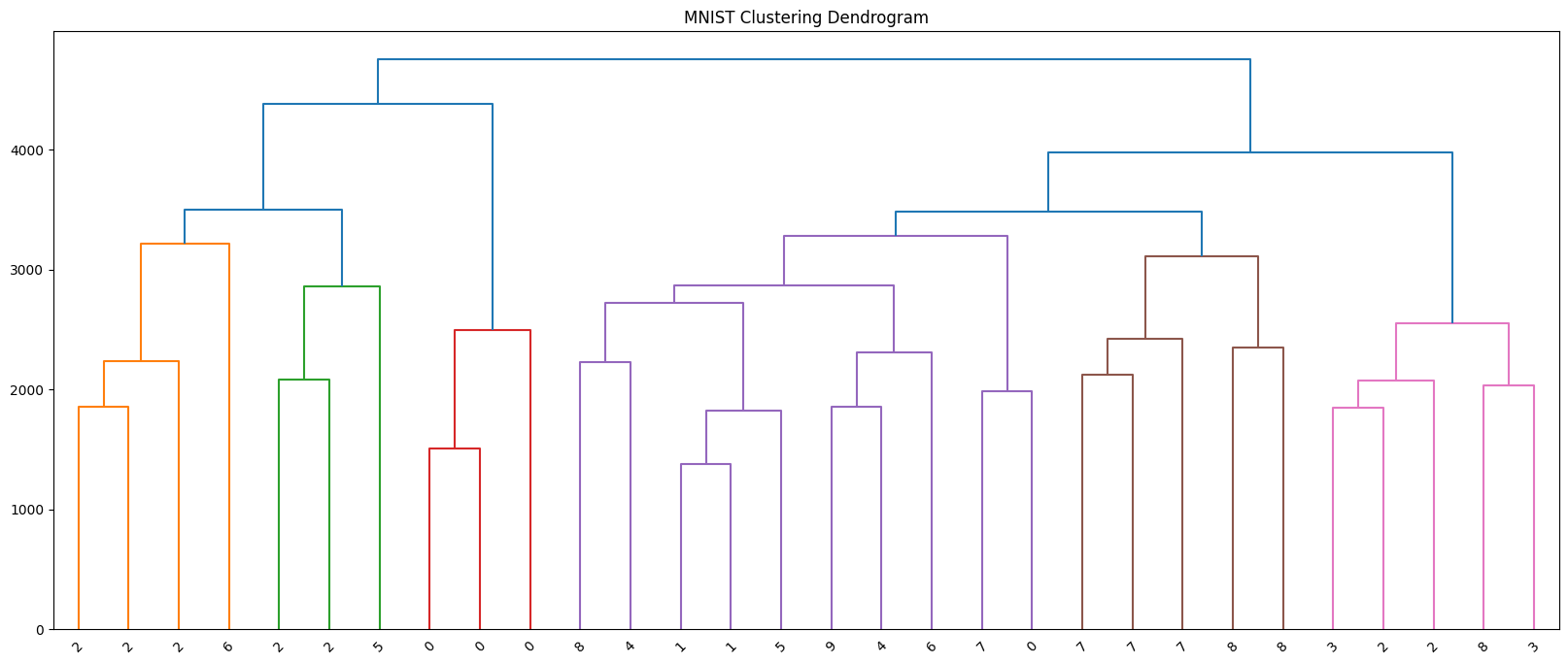
from torchvision.datasets import CIFAR10CIFAR-10 로드 + flatten 변환
# - 위에서 정의한 transforms:
#   v2.ToImage() -> (C,H,W) 텐서
#   v2.Lambda(torch.flatten) -> 1D 벡터로 펼침
# - CIFAR-10 테스트셋: 10,000장, 각 샘플은 (3,32,32) -> (3072,) 벡터

flatten_cifar10 = CIFAR10(".", train=False, download=True, transform=transforms)
# 임의로 30개 샘플 선택 (시드는 앞서 np.random.seed로 고정했다고 가정)
cifar10_indices = np.random.choice(len(flatten_cifar10), 30, replace=False)# X: (30, 3072) 실수 배열 / y: (30,) 정수 라벨(0~9: airplane~truck)
flatten_X = np.array([flatten_cifar10[idx][0].numpy() for idx in cifar10_indices])
flatten_y = np.array([flatten_cifar10[idx][1] for idx in cifar10_indices])Agglomerative Clustering
# - compute_distances=True: 병합 거리 저장(덴드로그램 그리기에 필요)
model = AgglomerativeClustering(compute_distances=True)
model = model.fit(flatten_X)
덴드로그램 시각화
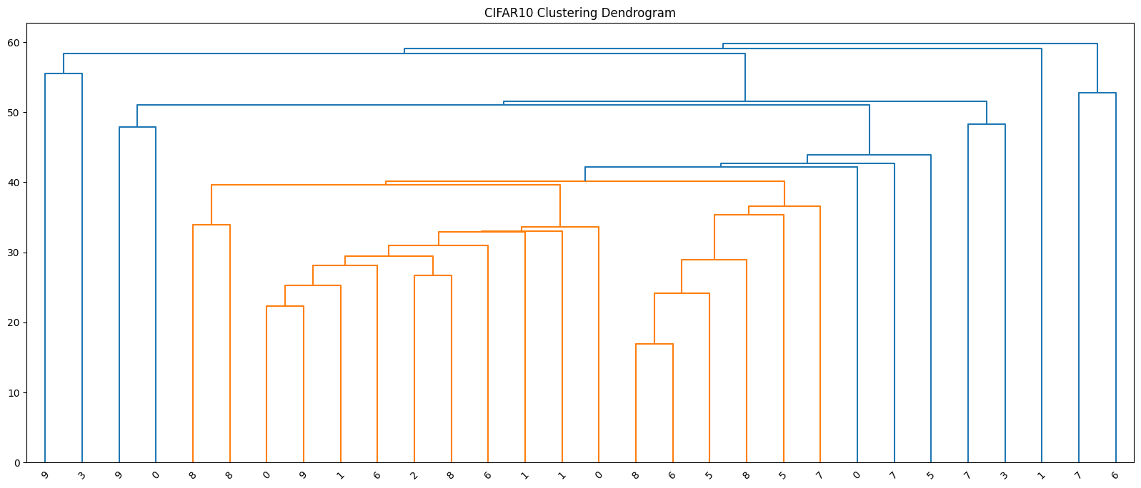
plt.figure(figsize=(20, 8))
plt.title("CIFAR10 Clustering Dendrogram")
plot_dendrogram(model, flatten_y) # x축 라벨로 실제 클래스 id 표시(0~9)
plt.show()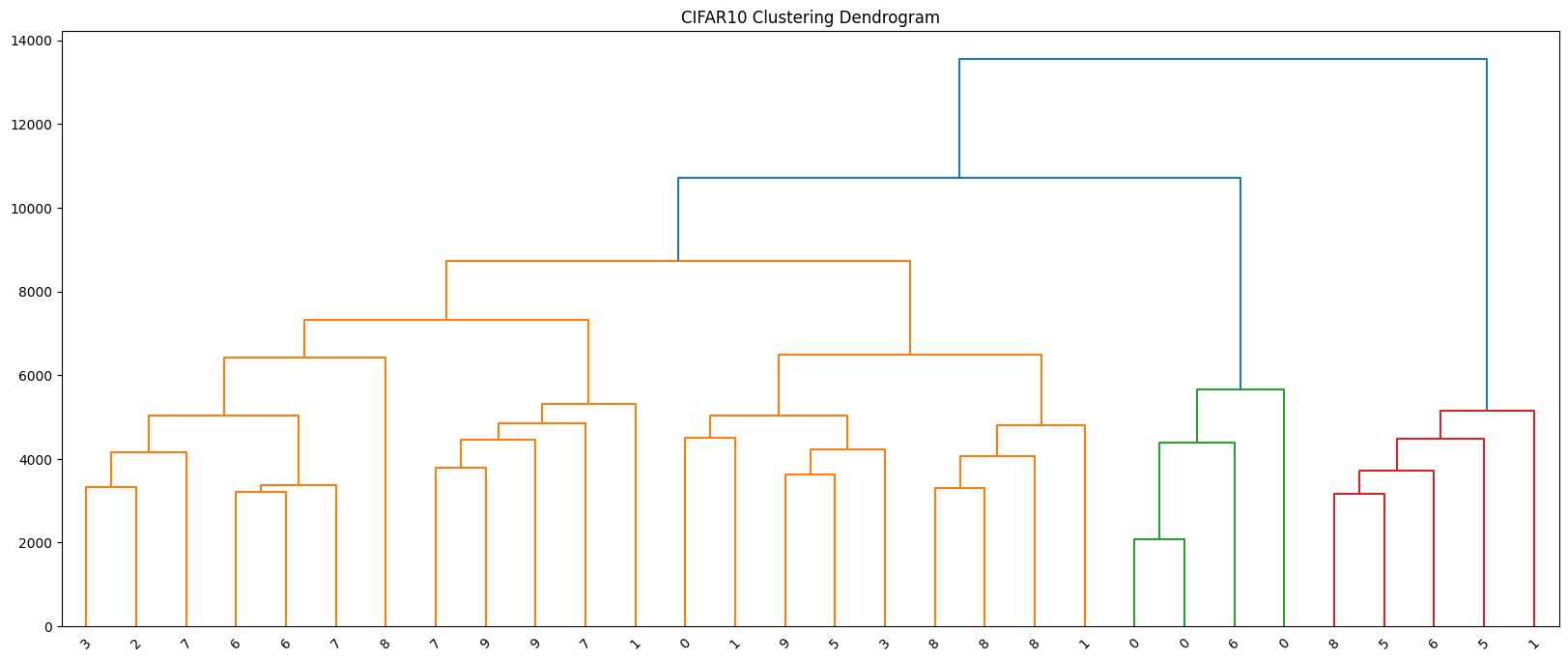
- 적절한 군집 수 k를 가늠할 수 있음
- 세로축(높이): 두 클러스터가 병합될 때의 거리. 세로로 큰 간격이 생기는 지점 바로 아래에 수평선을 그으면, 그 선과 만나는 가지 개수가 자연스러운 k가 됨
- 예) 세로가 3 -> 2개로 병합될 때 가장 큰 간격이 되었다면 k=3이 데이터 구조를 잘 설명 가능성이 큼
- 군집 간 유사도를 확인할 수 있음
- 높은 위치에서 합쳐지는 두 클러스터일수록 서로 멀고 구분이 잘 안된다는 뜻
- 낮은 높이에서 바로 합쳐지면 가깝고 비슷하다는 뜻
transforms = v2.Compose([
    v2.ToImage(), # (H,W,C) → torch.Tensor(C,H,W)
    v2.ToDtype(torch.float32, scale=True), # [0,255] → [0,1] + float32
    v2.Normalize(mean=[0.485, 0.456, 0.406], std=[0.229, 0.224, 0.225]), # ImageNet 평균/표준편차
])
# 테스트셋 로드 (변환 적용)
normal_cifar10 = CIFAR10(".", train=False, download=True, transform=transforms)normal_X = torch.stack([normal_cifar10[idx][0] for idx in cifar10_indices])
normal_y = np.array([normal_cifar10[idx][1] for idx in cifar10_indices])import torch.nn as nn
from torchvision.models import resnet18, ResNet18_Weights# ResNet18 백본으로 피처 추출
feature_extractor = resnet18(weights=ResNet18_Weights.DEFAULT) # ImageNet 사전학습 가중치
feature_extractor ResNet(
(conv1): Conv2d(3, 64, kernel_size=(7, 7), stride=(2, 2), padding=(3, 3), bias=False)
(bn1): BatchNorm2d(64, eps=1e-05, momentum=0.1, affine=True, track_running_stats=True)
(relu): ReLU(inplace=True)
(maxpool): MaxPool2d(kernel_size=3, stride=2, padding=1, dilation=1, ceil_mode=False)
(layer1): Sequential(
(0): BasicBlock(
(conv1): Conv2d(64, 64, kernel_size=(3, 3), stride=(1, 1), padding=(1, 1), bias=False)
(bn1): BatchNorm2d(64, eps=1e-05, momentum=0.1, affine=True, track_running_stats=True)
(relu): ReLU(inplace=True)
(conv2): Conv2d(64, 64, kernel_size=(3, 3), stride=(1, 1), padding=(1, 1), bias=False)
(bn2): BatchNorm2d(64, eps=1e-05, momentum=0.1, affine=True, track_running_stats=True)
)
(1): BasicBlock(
(conv1): Conv2d(64, 64, kernel_size=(3, 3), stride=(1, 1), padding=(1, 1), bias=False)
(bn1): BatchNorm2d(64, eps=1e-05, momentum=0.1, affine=True, track_running_stats=True)
(relu): ReLU(inplace=True)
(conv2): Conv2d(64, 64, kernel_size=(3, 3), stride=(1, 1), padding=(1, 1), bias=False)
(bn2): BatchNorm2d(64, eps=1e-05, momentum=0.1, affine=True, track_running_stats=True)
)
)
(layer2): Sequential(
(0): BasicBlock(
(conv1): Conv2d(64, 128, kernel_size=(3, 3), stride=(2, 2), padding=(1, 1), bias=False)
(bn1): BatchNorm2d(128, eps=1e-05, momentum=0.1, affine=True, track_running_stats=True)
(relu): ReLU(inplace=True)
(conv2): Conv2d(128, 128, kernel_size=(3, 3), stride=(1, 1), padding=(1, 1), bias=False)
(bn2): BatchNorm2d(128, eps=1e-05, momentum=0.1, affine=True, track_running_stats=True)
(downsample): Sequential(
(0): Conv2d(64, 128, kernel_size=(1, 1), stride=(2, 2), bias=False)
(1): BatchNorm2d(128, eps=1e-05, momentum=0.1, affine=True, track_running_stats=True)
)
)
(1): BasicBlock(
(conv1): Conv2d(128, 128, kernel_size=(3, 3), stride=(1, 1), padding=(1, 1), bias=False)
(bn1): BatchNorm2d(128, eps=1e-05, momentum=0.1, affine=True, track_running_stats=True)
(relu): ReLU(inplace=True)
(conv2): Conv2d(128, 128, kernel_size=(3, 3), stride=(1, 1), padding=(1, 1), bias=False)
(bn2): BatchNorm2d(128, eps=1e-05, momentum=0.1, affine=True, track_running_stats=True)
)
)
(layer3): Sequential(
(0): BasicBlock(
(conv1): Conv2d(128, 256, kernel_size=(3, 3), stride=(2, 2), padding=(1, 1), bias=False)
(bn1): BatchNorm2d(256, eps=1e-05, momentum=0.1, affine=True, track_running_stats=True)
(relu): ReLU(inplace=True)
(conv2): Conv2d(256, 256, kernel_size=(3, 3), stride=(1, 1), padding=(1, 1), bias=False)
(bn2): BatchNorm2d(256, eps=1e-05, momentum=0.1, affine=True, track_running_stats=True)
(downsample): Sequential(
(0): Conv2d(128, 256, kernel_size=(1, 1), stride=(2, 2), bias=False)
(1): BatchNorm2d(256, eps=1e-05, momentum=0.1, affine=True, track_running_stats=True)
)
)
(1): BasicBlock(
(conv1): Conv2d(256, 256, kernel_size=(3, 3), stride=(1, 1), padding=(1, 1), bias=False)
(bn1): BatchNorm2d(256, eps=1e-05, momentum=0.1, affine=True, track_running_stats=True)
(relu): ReLU(inplace=True)
(conv2): Conv2d(256, 256, kernel_size=(3, 3), stride=(1, 1), padding=(1, 1), bias=False)
(bn2): BatchNorm2d(256, eps=1e-05, momentum=0.1, affine=True, track_running_stats=True)
)
)
(layer4): Sequential(
(0): BasicBlock(
(conv1): Conv2d(256, 512, kernel_size=(3, 3), stride=(2, 2), padding=(1, 1), bias=False)
(bn1): BatchNorm2d(512, eps=1e-05, momentum=0.1, affine=True, track_running_stats=True)
(relu): ReLU(inplace=True)
(conv2): Conv2d(512, 512, kernel_size=(3, 3), stride=(1, 1), padding=(1, 1), bias=False)
(bn2): BatchNorm2d(512, eps=1e-05, momentum=0.1, affine=True, track_running_stats=True)
(downsample): Sequential(
(0): Conv2d(256, 512, kernel_size=(1, 1), stride=(2, 2), bias=False)
(1): BatchNorm2d(512, eps=1e-05, momentum=0.1, affine=True, track_running_stats=True)
)
)
(1): BasicBlock(
(conv1): Conv2d(512, 512, kernel_size=(3, 3), stride=(1, 1), padding=(1, 1), bias=False)
(bn1): BatchNorm2d(512, eps=1e-05, momentum=0.1, affine=True, track_running_stats=True)
(relu): ReLU(inplace=True)
(conv2): Conv2d(512, 512, kernel_size=(3, 3), stride=(1, 1), padding=(1, 1), bias=False)
(bn2): BatchNorm2d(512, eps=1e-05, momentum=0.1, affine=True, track_running_stats=True)
)
)
(avgpool): AdaptiveAvgPool2d(output_size=(1, 1))
(fc): Linear(in_features=512, out_features=1000, bias=True)
)# 모델의 fc 층을 아무 연산도 하지 않는 층으로 교체
# 파라미터 없음, 연산 없음
# 피처 추출 전용(backbone)으로 사용하기 위함
feature_extractor.fc = nn.Identity()feature_X = feature_extractor(normal_X).detach().numpy()
feature_Xarray([[1.3213383 , 0.84684217, 1.0053906 , ..., 0.83199936, 0. ,
0.6355228 ],
[0. , 0. , 0. , ..., 8.524711 , 3.7137005 ,
0. ],
[0.515726 , 0. , 0. , ..., 0.32266223, 1.4728183 ,
0. ],
...,
[0.5772192 , 0.7121287 , 0.01978162, ..., 0.65148675, 1.3684964 ,
1.4148082 ],
[0.7430557 , 0. , 2.0633652 , ..., 0.5895468 , 0.6749586 ,
0. ],
[0. , 0. , 5.1838355 , ..., 0. , 0. ,
0. ]], dtype=float32)계층적(병합) 클러스터링 모델
# compute_distances=True: 각 병합 단계의 거리 기록
model = AgglomerativeClustering(compute_distances=True)
# 피처 벡터로 트리(병합 히스토리) 학습
model = model.fit(feature_X)
덴드로그램 시각화
plt.figure(figsize=(20, 8))
plt.title("CIFAR10 Clustering Dendrogram")
plot_dendrogram(model, normal_y)
plt.show()