4.1 Why Linearization?
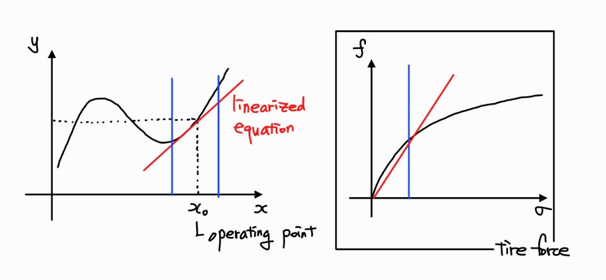
Linearization(선형화) 란 어떤 비선형 시스템을 근사하는 선형 모델을 찾는 과정이다. 대부분 현실 세계의 물리 시스템은 비선형적이다. 그런데 본래 비선형 시스템인 것을 operating point 근처에서 선형화하여 local dynamic behavior을 조사하는 것이 합리적이다. 이를 위해, 라플라스 변환이나 선형대수 등 선형 시스템을 분석하는 데 유용한 수학적 툴이 존재한다.
Recall: Basic Characteristics of Lienar System - Superposition

4.2 Linearization using Taylor Series Expansion
y=f(x)=f(x0)+dxdf∣∣∣∣x0(x−x0)+2!1dx2d2f∣∣∣∣x0(x−x0)2+3!1dx(3)d(3)f∣∣∣∣x0(x−x0)3+⋯
x−x0가 매우 작으면
y≃f(x0)+dxdf∣∣∣∣x0(x−x0)
Example: Rotational pendulum
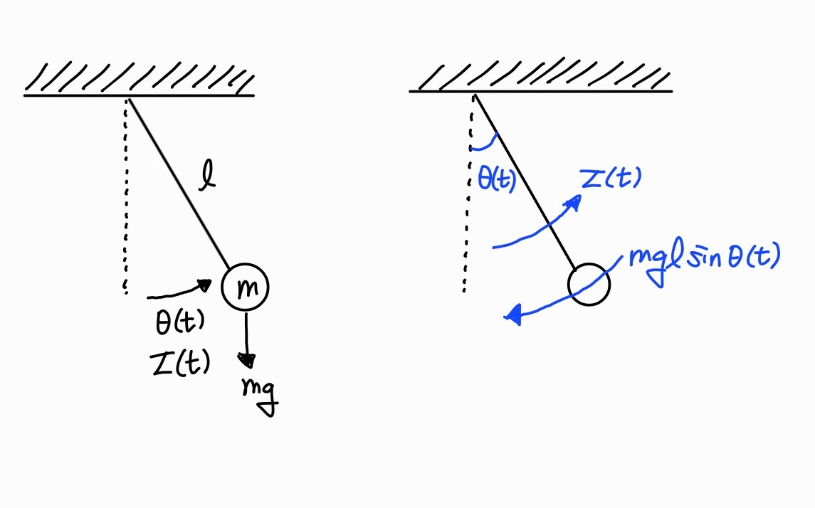
τ(t)−mglsinθ(t)=Jα=ml2θ¨(t)
⇔ml2θ¨(t)+mglsinθ(t)=τ(t)
⇔θ¨(t)+lgsinθ(t)=ml2τ(t) ← 여전히 비선형 모델(①)
만약 motion이 매우 작다면, sinθ(t)≈θ(t)라고 할 수 있다.
Taylor 급수를 활용하여 θ0=0 부근에서 비선형 함수를 선형화한다고 하자. 비선형 함수 y=lgsinθ(t)에 대해,
y≈(x0)+dxdf∣∣∣∣x0(x−x0)=lgsin(θ0)+lgcos(θ0)(θ(t)−θ0)=lgθ(t)
①은 다음과 같이 선형화할 수 있다.
θ¨(t)+lgθ(t)=ml2τ(t)
4.3 Solution of Differential Equations of Dynamic Systems
4.3.1 Response

mx¨(t)+bx˙(t)+kx(t)=f(t)
시스템의 시간 영역에서 특정 입력에 대한 응답은 무엇인가? 그전에 몇몇 중요한 입력 신호를 살펴볼 필요가 있다.
Unit Step Function
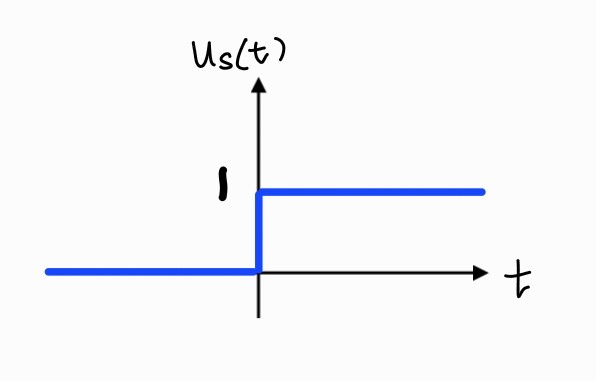
us(t)={10t≥0otherwise
Unit Ramp Function
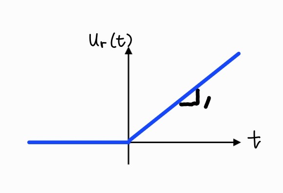
ur(t)={t0t≥0otherwise
(ideal) Impulse Function(or Dirac Delta Function)
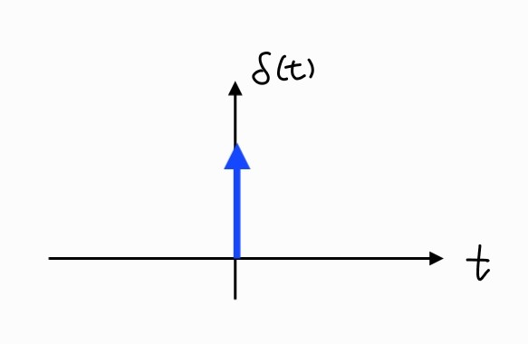
ui(t)=δ(t)=0,t=0
∫−∞∞δ(x)dx=1
Sifting Property: ∫−∞∞x(τ)δ(t−τ)dτ=x(t)
입력 x(t)을 가지는 LTI 시스템의 출력을 y(t)라 하자.
y(t)=T[x(t)]
sifting → T[∫−∞∞x(τ)δ(x−τ)dτ]
linear → ∫−∞∞x(τ)T[δ(x−τ)]dτ
h(t−τ)=T[δ(t−τ)]라고 하면
convolution integral → ∫−∞∞x(τ)h(t−τ)dτ
∴y(t)≜x(t)∗h(t)
따라서 LTI 시스템에서는, impulse response을 안다면 컨볼루션 적분만으로 어느 입력값에 대해서든 출력 응답을 찾을 수 있다.
Example: Find a impulse response
First order system 하나를 보자.
y˙(t)+ky(t)=u(t)
y(0−)=0라 하면, u(t)=δ(t)이다.
t>0에 대해, y˙(t)+ky(t)=0⇔y(t)=Aest,y˙(t)=Asest
⇒Asest+kAest=0
여기서, s=−k라 하고,
∫0−0+y˙(t)dt+k∫0−0+y(t)dt=∫0−0+δ(t)dt
⇔y(0+)−y(0−)+0=1
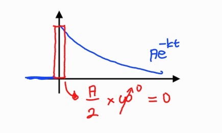
h(t)={e−kt0t≥0t<0or e−ktus(t)
Response of this system to general input
y(t)=∫−∞∞h(τ)u(t−τ)dτ=∫−∞∞e−ktus(τ)u(t−τ)dτ=∫0∞e−ktu(t−τ)dτ
4.3.2 How to find Impulse response experimentally?
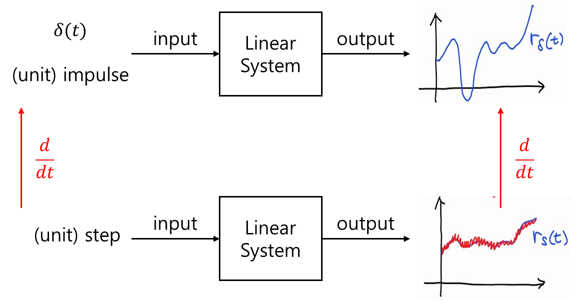
단위 임펄스 입력 대신, 단위 계산 입력을 적용한 후, 출력 응답을 시간에 대해 미분하여 구하는 것이다. 한편, 실험적으로 시스템의 응답을 구할 때는, 실제 환경에서 잡음이 필연적으로 발생하며, 이 잡음이 출력 응답을 왜곡할 수 있다.
ru=u∗rs˙(t)=u˙rs(t)
Recall - RLC network
LCdt2d2eC(t)+RCdtdeC(t)+eC(t)=e(t)
Recall - Mass-spring-damper system
Mdt2d2x(t)+βdtdx(t)+kx(t)=f(t)
Standard second order system of form
y¨(t)+2ζwny˙(t)+wn2y(t)=wn2u(t)
일반적으로, n차 선형 상미분 방정식(linear ordinary differential equation of nth order)은 다음과 같이 쓰인다.
dtndny(t)+an−1dtn−1dn−1y(t)+⋯+a1dtdy(t)+a0y(t)=bmdtmdmu(t)+bm−1dtm−1dm−1u(t)+⋯+b1dtdu(t)+b0u(t)
라플라스 변환은 선형 미분 방정식을 풀기 위한 하나의 방법이다. 이는 선형 상미분 방정식을 대수 방정식으로 변환시킨다.
함수 f(t)에 대한 라플라스 변환은 다음과 같이 정의된다.
F(s)=∫0−∞f(x)e−stdx=L[f(t)]
여기서 변수 s(=σ+jw)은 Laplace operator로 불린다.

다양한 신호에 대해 라플라스 변환을 해보겠다.
step function
us(t)={A0t≥0otherwise⇒L[us(t)]=sA
Ramp function
ur(t)={At0t≥0otherwise⇒L[ur(t)]=s2A
Pulse function: ① + ②
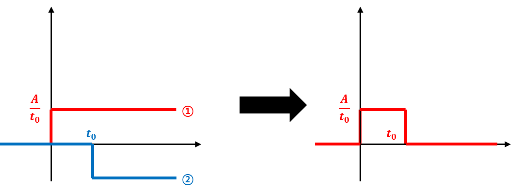
up(t)={t0A00≤t<t0otherwise⇒L[up(t)]=st0A(1−e−st0)
Impulse function
ui(t)={limt0→0t0A00≤t<t0otherwise⇒L[ui(t)]=A
Example: Laplace transform of a unit step function
F(s)=L[us(t)]=∫0∞us(t)e−stdt=∫0∞1⋅e−stdt=−s1e−st∣∣∣0∞=−s1⋅0−(−s1⋅1)=s1
Example: Laplace transform of an exponential function
f(t)=e−at,t>0
F(s)=L[f(t)]=∫0∞e−at⋅e−stdt=∫0∞e−(s+a)tdt=−s+a1e−(s+a)t∣∣∣0∞=s+a1
라플라스 변환은 다음의 특성을 가진다.
- Linearity
L[Af(t)]=AF(s)
L[f1(t)+f2(t)]=F1(s)+F2(s)
- Delay
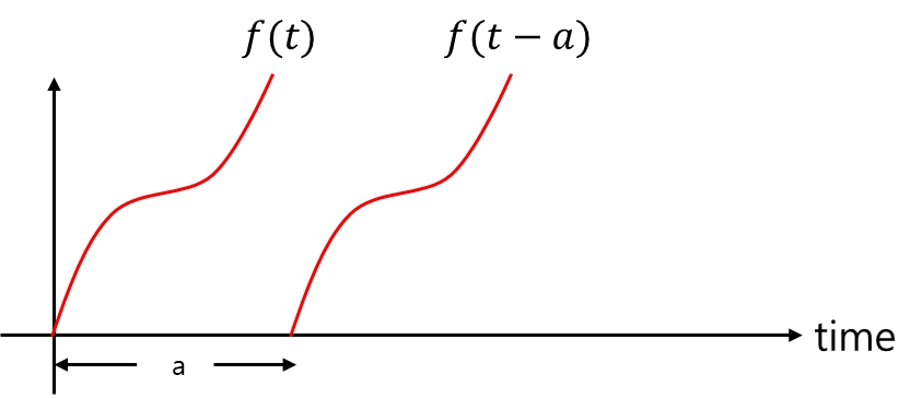
L[f(t−a)]=e−saF(s)
- Differentiation
L[f(t)]=F(s)
L[dtdf(t)]=sF(s)−f(0)
L[dt2d2f(t)]=s2F(s)−sf(0)−f˙(0)
⋯
L[dtndnf(t)]=snF(s)−sn−1f(0)−sn−2f(1)(0)−sn−3f(2)(0)−⋯−f(n−1)(0)
where f(n)(0)=dtndnf(t)∣∣∣∣t=0
Proof)
L[dtdf(t)]=∫0∞dtdf(t)e−stdt=∫0∞e−stdtdf(t)dt
※ 부분적분법
∫abu(t)⋅v˙(t)dt=u(t)v(t)∣ab−∫abu˙(t)v(t)dt
여기서는 u(t)=e−st,v(t)=f(t)이다.
그에 따라
∫0∞e−stdtdf(t)dt=e−stf(t)∣0∞−∫0∞−ste−stf(t)dt=−f(0)+s∫0∞e−stf(t)dt=F(s)−f(0)
또한,
L[f¨(t)]=sL[f(t)˙]−f˙(0)=s(sF(s)−f(0))−f˙(0)=s2F(s)−sf(0)−f˙(0)
- Integration
L[∫0tf(τ)dτ]=sF(s)