Introduction

As AI models get bigger and deeper, understanding how AI model works has been a growing topic among many researchers. A few researches focus on layer-wise interpretation of the deep audio features (Shim et al (2022, ICLR), Pasad et al (2021, ASRU)). However, audio domain is inherently hard to interpret due to its relatively counter-intuitive data formats such as Mel spectrograms or Mel-Frequency Cepstral Coefficients, and more. Experts in speech processing might be able to recognize some bits of high-level information (Phoneme, Prosody, etc) just by seeing the raw spectrogram alone, which is not a case in most people.

This paper (Paissan et al., 2024, ICML (Oral)), referred to as L-MAC (Listenable Maps for Audio Classifiers) is a novel introducive research to understanding the 'difficult' audio data through the scope of audio classification.

Methodology

This paper focuses on understanding the understandability of the audio representation, and CLAP (Contrastive Language-Audio Pretraining) is selected as a baseline classifier.

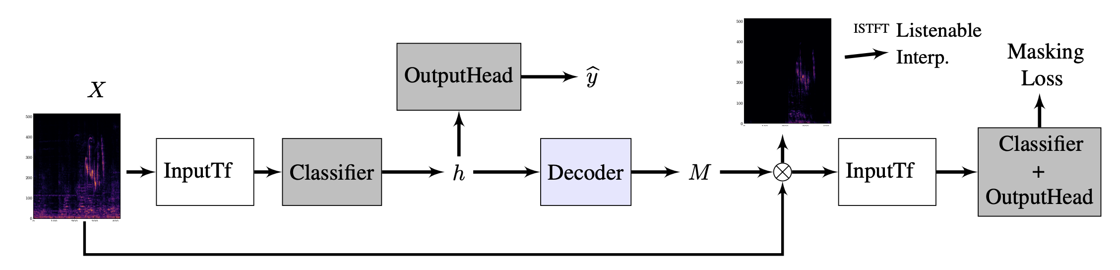
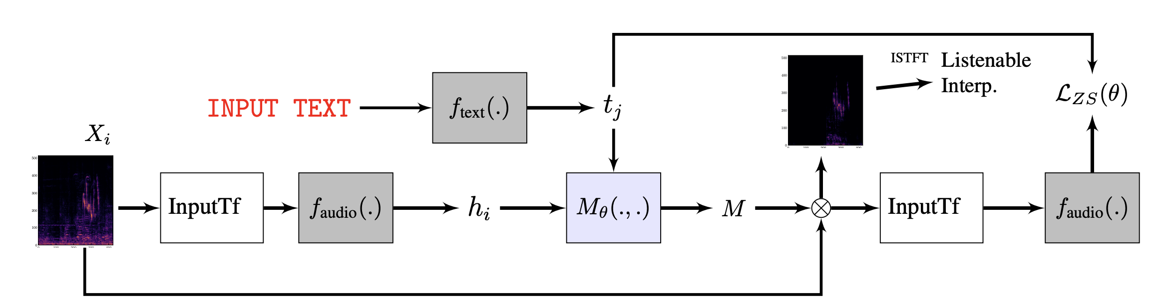
Let me break down the illustration above into smaller segments.

1. The input linear spectrogram $X$ is computed from the audio waveform $x$, processed into a desired type of feature in a baseline audio classifiers (log-mel filterbanks usually). Then the input data is fed into the audio classifier $f_{audio}()$ to generate the latent representation $h$.

   Latent representation $h$ is usually fed to a linear layer to output a probability of a class distribution in an application, which is not the case here because we only need the latent representation $h$.

2. Next up, the representation $h$ is fed into the decoder, which is trained to generate a binary mask $M$ most relevant to predicting the class information.

   $M = dec (h)$

How is $M$ predicted?

Well, this is the most important aspect of the paper and the very novelty that the research focuses on.

The basic intuition behind $M$ is that the classifier should make a good classification (maximize the confidence of the classification decision) with the masked-in-portion of the audio, while should make a poor decision for the masked-out portion.

Masking objective $M$ is a binary mask that is shaded on the linear spectrogram with a binary objective of 0 when masked, 1 when not masked.

On the loss function above, $M \cdot X$ produces a masked linear spectrogram and $f$ serves as a classifier. $L_{in}$ is the categorical cross-entropy loss computed for the masked input. The interesting part is that $y$ is not a ground truth label but the prediction of the classifier with the full (unmasked) input $argmax \ f(X)$. The interpretation not only cares about the correct answer but focues slightly more on how the classifier changes its decision when some portions are given.

Since $(1-M) \cdot X$ represents the part that is not selected by the mask $M$, We want the cross-entropy between the part of $(1-M) \cdot X$ and $y$ to be high, meaning that the model gets difficult when given with the masked-out portion of the data. Lastly, the regularizer $R(M)$ works as a $L1$ distance limiter to ensure that not too much of a masked portion can grow.

Producing Listenable Explanations

The primary reason LMAC separates the use of linear spectrogram and mel filterbanks is that only linear spectrogram with both the maginitude and phase allows for us the use of Inverse Short-Time Fourier Transform (ISTFT) to make a listenable maps. The time-domain audio signal is made through:

$x_{interpretation} = ISTFT((M(h)\cdot X)e^{jX_{phase}})$ where $j$ is an imaginary nnumber.

Results

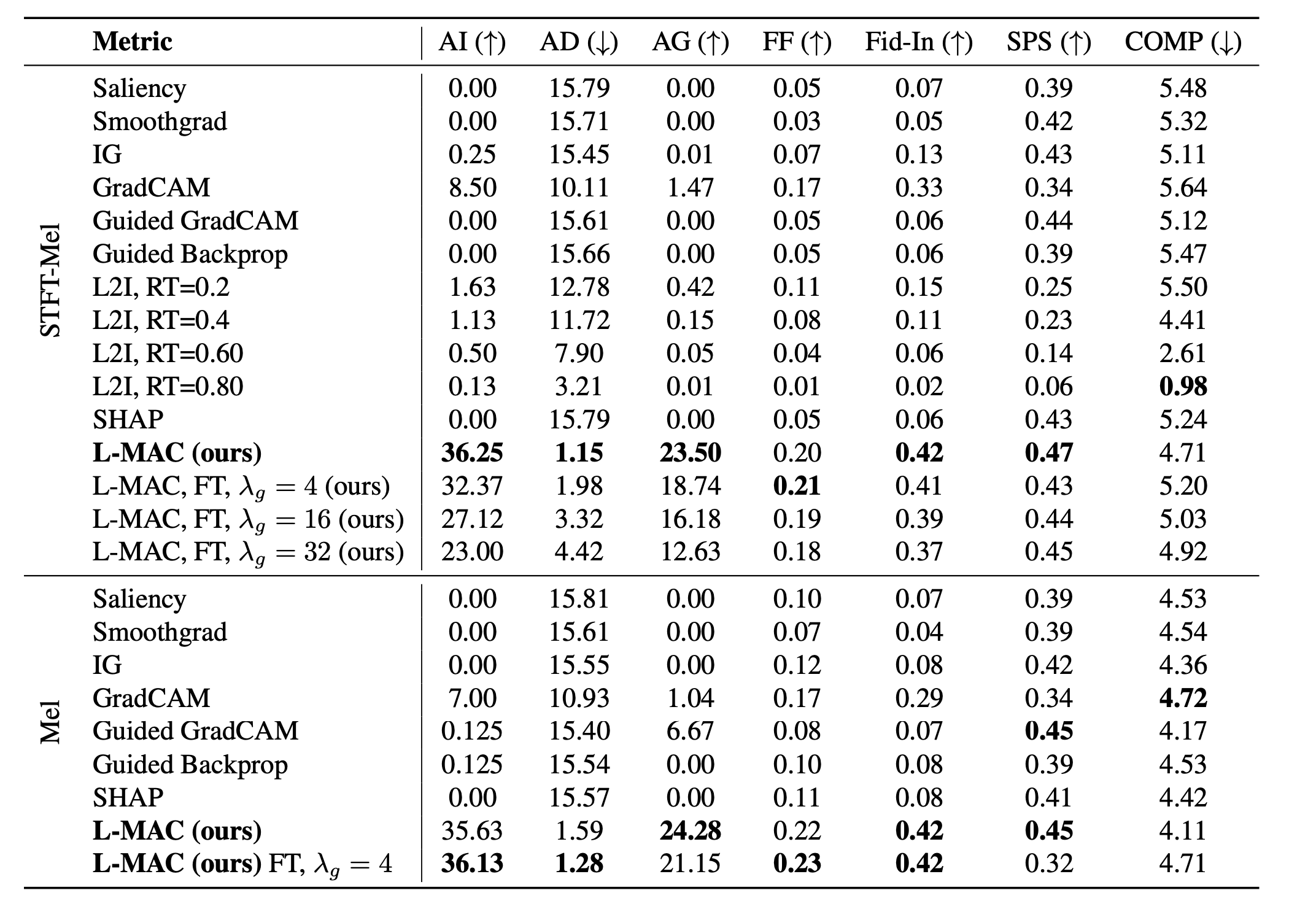
You can look at the paper for the very details of the experiments or the metrics one by one.