Contents Based Filtering
-
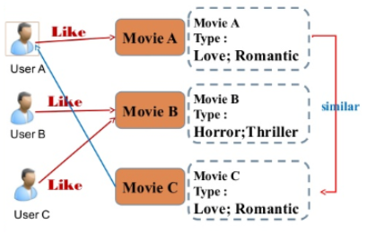
아이템에 대한 메타 데이터를 이용하여 어떤 사람이 특정 아이템을 선호한다면, 그것과 비슷한 아이템을 추천하는 방식
- ex) 영화의 content(overview, cast, crew, keyword, tagline etc)를 사용하여 유사한 영화를 추천
-
장점: 사용자가 평점을 매기지 않은 새로운 아이템이 들어와도 추천이 가능함
-
단점
- 기존 아이템과 유사한 아이템 위주로만 추천, 새로운 장르의 아이템을 추천하기 어려움
- 아이템의 피쳐를 추출해야하는데, 제대로 피쳐를 추출하지 못하면 성능이 낮음.
데이터셋
- tmdb dataset을 사용하며, 2개로 분리되어 있는 dataset을 id(movie_id)로 join하여 사용
import pandas as pd
import numpy as np
df1=pd.read_csv('../input/tmdb-movie-metadata/tmdb_5000_credits.csv')
df2=pd.read_csv('../input/tmdb-movie-metadata/tmdb_5000_movies.csv')
df1.columns = ['id','tittle','cast','crew']
df2= df2.merge(df1,on='id')
The first dataset contains the following features:
- movie_id - A unique identifier for each movie.
- cast - The name of lead and supporting actors.
- crew - The name of Director, Editor, Composer, Writer etc.
The second dataset has the following features:-
- budget - The budget in which the movie was made.
- genre - The genre of the movie, Action, Comedy ,Thriller etc.
- homepage - A link to the homepage of the movie.
- id - This is infact the movie_id as in the first dataset.
- keywords - The keywords or tags related to the movie.
- original_language - The language in which the movie was made.
- original_title - The title of the movie before translation or adaptation.
- overview - A brief description of the movie.
- popularity - A numeric quantity specifying the movie popularity.
- production_companies - The production house of the movie.
- production_countries - The country in which it was produced.
- release_date - The date on which it was released.
- revenue - The worldwide revenue generated by the movie.
- runtime - The running time of the movie in minutes.
- status - "Released" or "Rumored".
- tagline - Movie's tagline.
- title - Title of the movie.
- vote_average - average ratings the movie recieved.
- vote_count - the count of votes recieved.
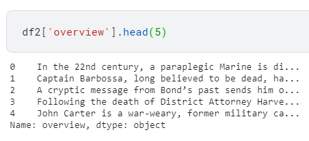
- df2 DataFrame의 "overview" column은 아래와 같다.
임베딩 방법
- NLP에서 사용하는 Word2Vec 방법들은 별도 포스트로 작성
- ex) CBOW, Skip-gram, SGNS(Skip-gram Negative Sampling)
TF-IDF
- TF-IDF (Term Frequency-Inverse Document Frequency)
- 문서(예제 기준으로는 영화)를 Vector로 나타내는 방법으로, TF * IDF를 계산한다.
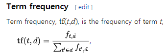
- Term Frequency: 특정 문서 d에서의 특정 단어 t의 등장 횟수
- Document Frequency: 특정 단어 t가 등장한 문서의 수
- Inverse Document Frequency: DF에 반비례하는 수
- n: 문서의 수
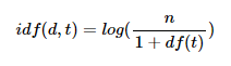
- n: 문서의 수
- Term Frequency: 특정 문서 d에서의 특정 단어 t의 등장 횟수
- scikit-learn에 CountVectorizer, TF-IDF 등이 구현되어 있으며, 아래와 같이 사용
- 불용어(stop_words)를 제거하는 목적으로 TfidfVectorizer의 stop_words 인수를 사용
- 4,803개의 movie overview에서 stop_words를 제외한 20,978개의 words가 사용되었음.
from sklearn.feature_extraction.text import TfidfVectorizer

tfidf = TfidfVectorizer(stop_words='english')
df2['overview'] = df2['overview'].fillna('') # NaN을 empty string으로 대체
tfidf_matrix = tfidf.fit_transform(df2['overview']) #fit 이후, TF-IDF matrix로 변환(transform)
tfidf_matrix.shape # (4803, 20978)
유사도 계산
-
위에서 TF-IDF를 통해 얻은 matrix로 유사도를 계산할 수 있음
-
Euclidean(유클리디안), Pearson(피어슨), Cosine(코사인) 등과 같은 후보가 있으며, 어떤 것이 가장 좋다고 정해진 것은 없음
-
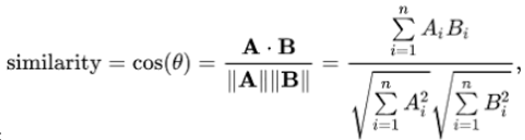
여기서는 코사인 유사도를 사용
-
유사도 함수들 또한 sklearn에 구현되어 있으며, 아래와 같이 사용
from sklearn.metrics.pairwise import linear_kernel
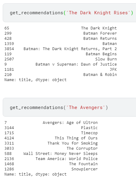
cosine_sim = linear_kernel(tfidf_matrix, tfidf_matrix)- 계산된 각 영화 간의 유사도를 통해, 어떤 사람이 특정 영화를 선호할 때 유사한 top 10을 추천
indices = pd.Series(df2.index, index=df2['title']).drop_duplicates() # 영화 제목 => matrix의 인덱스 맵핑 목적

def get_recommendations(title, cosine_sim=cosine_sim):
    idx = indices[title]
    sim_scores = list(enumerate(cosine_sim[idx]))
    sim_scores = sorted(sim_scores, key=lambda x: x[1], reverse=True)
    sim_scores = sim_scores[1:11]
    movie_indices = [i[0] for i in sim_scores]
return df2['title'].iloc[movie_indices]- 추천 결과
기타 메타데이터를 이용한 방법
- 해당 Notebook에서는
Credits(Cast, Director), Genres, Keyword메타데이터를 사용하여 embedding 한 후 추천하는 방법도 제시하고 있음.
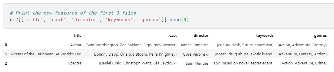
- metadata soup(아마 여러 메타데이터가 섞여있어서 수프라고 함)를 만들어서 사용
def create_soup(x):
    return ' '.join(x['keywords']) + ' ' + ' '.join(x['cast']) + ' ' + x['director'] + ' ' + ' '.join(x['genres'])
df2['soup'] = df2.apply(create_soup, axis=1)- 한 가지 다른 점으로는 TF-IDF를 사용하지 않고, CountVectorizer를 사용
- TF-IDF를 사용하면 actor/director 메타데이터의 경우 상대적으로 down-weight 되기 때문
from sklearn.feature_extraction.text import CountVectorizer

count = CountVectorizer(stop_words='english')
count_matrix = count.fit_transform(df2['soup'])
Collaborative Filtering
Neighborhood Based
-
Neighborhood Based Collaborative Filtering 으로 User Based, Item Based가 있음
-
단점
- 유저의 성향은 계속 바뀔 수 있음
- 시간, 속도, 메모리가 많이 필요 (많은 유저들 간에 유사도를 계산해야 하므로)
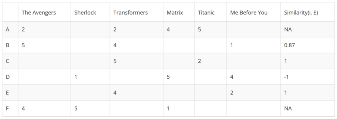
User Based
- User Based Collaborative Filtering은 각 유저의 선호도 데이터에서, 각 유저(User)에 대한 유사도를 계산
- 아래 예제에서는 Target인
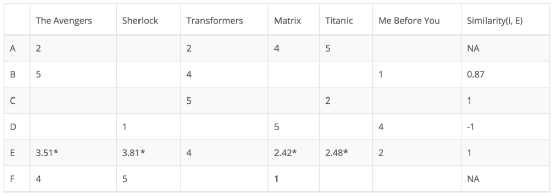
E와의 유사도를 계산함- 알고 싶은 E의 빈칸은 나와 유사한 k개의 유저에서 아래처럼 계산 (KNN)
- (Σ유사한 User의 평점 * 유사도값)/(Σ유사도값)을 이용함
- E의 빈칸인 각 영화에 대한 예상 선호도를 알 수 있으며, 이를 기반으로 추천
- 알고 싶은 E의 빈칸은 나와 유사한 k개의 유저에서 아래처럼 계산 (KNN)
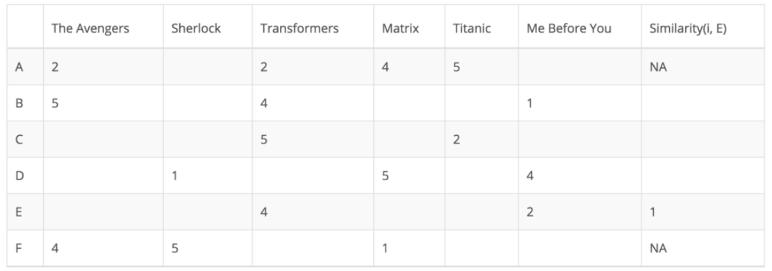
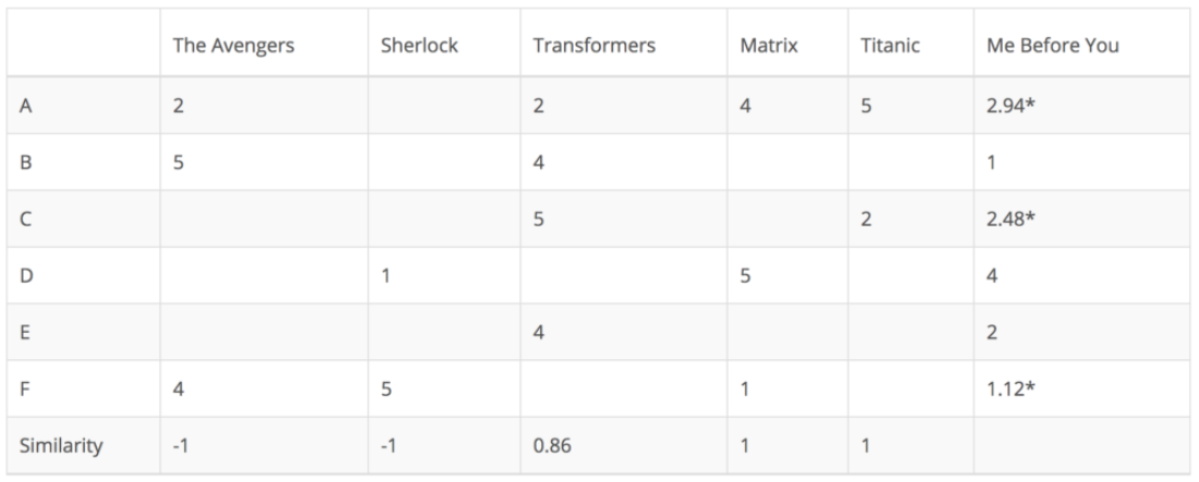
Item Based
- Item Based Collaborative Filtering은 각 유저의 선호도 데이터에서 각 영화(Item)에 유사도를 계산
- 아래 예제에서는 Target인
Me Before You영화와의 유사도를 계산함
Latent Factor Collaborative Filtering
- Rating Matrix의 빈 공간을 채우기 위해, 유저와 아이템을 잘 표현하는 Latent Factor를 찾는 방법
- 대표적인 방법으로 Matrix Factorization
- Matrix Factorization의 세부적인 방법으로는 아래와 같은 방법이 있음
- SVD(Single Value Decomposition)
- SGD(Stochastic Gradient Descent)
- ALS(Alternating Least Squares)
SGD
- 1.User Latent와 Item Latent를 랜덤값으로 초기화
- 2.User Latent x Item Latent 매트릭스를 이용하여 Rating Matrix를 예측하도록 학습
- 빈 공간(유저의 평점 데이터가 없는 경우)은 학습에서 제외
- 여러가지 Loss function을 사용해볼 수 있음
- 3.학습 완료 시, User Latent x Item Latent 매트릭스로 Rating Matrix의 빈 공간을 얻어 추천에 사용
ALS
- ALS는 User Latent와 Item Latent를 번갈아가며 고정 및 학습시키는 방법
- 1.User Latent와 Item Latent를 랜덤값으로 초기화
- 2.Item Matrix를 고정하고 User Matrix를 최적화
- 3.User Matrix를 고정하고 Item Matrix를 최적화
- 4.위 2~3의 과정을 반복하고 학습 완료 시 SGD와 동일하게 Rating Matrix를 얻어서 추천에 사용
Reference
- ✔ Kaggle Notebook: Getting Started with a Movie Recommendation System
- ✔ T academy 추천시스템 분석

개인 학습 및 복습을 위한 머신러닝 엔지니어의 블로그입니다 :)