1. 정리 범위
- 기준 모델과 여러 회귀 모델을 비교하는 방법
- 결정트리 회귀의 분할 원리와 하이퍼파라미터 튜닝
- 실제값과 예측값을 시각화해 오차를 확인하는 방법
- 시간 흐름에 따른 예측 결과 비교
- 트리 계열 모델의 피처 중요도와 결정트리 구조 해석
2. 여러 회귀 모델을 비교하는 이유
하나의 모델만 사용하면 그 모델의 성능이 좋은지 판단하기 어렵다. 먼저 평균만 예측하는 기준 모델을 만들고, 선형 모델과 트리·앙상블 모델을 같은 학습·테스트 데이터에서 평가해야 한다.
from sklearn.dummy import DummyRegressor
from sklearn.ensemble import (
    GradientBoostingRegressor,
    HistGradientBoostingRegressor,
    RandomForestRegressor,
)
from sklearn.linear_model import LinearRegression, Ridge
from sklearn.pipeline import Pipeline
from sklearn.tree import DecisionTreeRegressor

RANDOM_STATE = 2026

models = {
    "Dummy": Pipeline([
        ("preprocess", preprocess_for_tree),
        ("model", DummyRegressor(strategy="mean")),
    ]),
    "LinearRegression": Pipeline([
        ("preprocess", preprocess_for_linear),
        ("model", LinearRegression()),
    ]),
    "Ridge": Pipeline([
        ("preprocess", preprocess_for_linear),
        ("model", Ridge(alpha=1.0)),
    ]),
    "DecisionTree": Pipeline([
        ("preprocess", preprocess_for_tree),
        ("model", DecisionTreeRegressor(
            random_state=RANDOM_STATE,
        )),
    ]),
    "RandomForest": Pipeline([
        ("preprocess", preprocess_for_tree),
        ("model", RandomForestRegressor(
            random_state=RANDOM_STATE,
            n_estimators=300,
            n_jobs=-1,
        )),
    ]),
    "GradientBoosting": Pipeline([
        ("preprocess", preprocess_for_tree),
        ("model", GradientBoostingRegressor(
            random_state=RANDOM_STATE,
        )),
    ]),
    "HistGradientBoosting": Pipeline([
        ("preprocess", preprocess_for_tree),
        ("model", HistGradientBoostingRegressor(
            random_state=RANDOM_STATE,
        )),
    ]),
}| 모델 | 역할과 특징 |
|---|---|
DummyRegressor | 모든 행에 학습 데이터의 평균 대여량을 예측하는 기준선이다. |
LinearRegression | 입력 변수와 대여량이 하나의 선형 관계라고 가정한다. |
Ridge | 선형 회귀의 계수가 과도하게 커지지 않도록 규제를 적용한다. |
DecisionTreeRegressor | 조건에 따라 데이터를 나누고, 리프의 평균값으로 예측한다. |
RandomForestRegressor | 여러 트리의 예측을 평균내어 단일 트리의 불안정성을 줄인다. |
GradientBoostingRegressor | 이전 트리의 오차를 다음 트리가 순차적으로 보완한다. |
HistGradientBoostingRegressor | 연속형 값을 구간으로 묶어 부스팅 계산을 효율화한다. |
RandomForest는 여러 트리를 독립적으로 학습한 뒤 평균을 낸다. 반면 GradientBoosting은 앞 모델이 틀린 부분을 다음 모델이 학습하는 순차적인 방식이다.
3. 공통 평가와 모델 선택
각 모델은 같은 X_train, y_train으로 학습하고 같은 테스트 데이터로 평가한다. 47일차에서 만든 evaluate_regression() 함수는 MAE, MSE, RMSE, R2를 반환한다.
results = []

for name, model in models.items():
    model.fit(X_train, y_train)
    results.append(
        evaluate_regression(model, X_test, y_test, name)
    )

result_df = (
    pd.DataFrame(results)
    .sort_values("RMSE")
    .reset_index(drop=True)
)

print(result_df)
실행 결과
| 모델 | MAE | MSE | RMSE | R2 |
|---|---|---|---|---|
| RandomForest | 248.69 | 116,676.96 | 341.58 | 0.6752 |
| HistGradientBoosting | 260.74 | 116,687.54 | 341.60 | 0.6751 |
| DecisionTree | 280.76 | 149,756.22 | 386.98 | 0.5831 |
| GradientBoosting | 291.46 | 154,978.54 | 393.67 | 0.5685 |
| Dummy | 491.51 | 402,474.39 | 634.41 | -0.1205 |
| Ridge | 593.57 | 508,831.06 | 713.32 | -0.4166 |
| LinearRegression | 606.01 | 527,109.85 | 726.02 | -0.4675 |
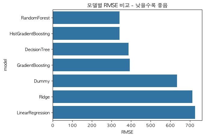
이번 실행에서는 RandomForest가 RMSE 341.58로 가장 낮고 R2 0.6752로 가장 높다. 트리 계열 모델이 선형 모델보다 좋은 결과를 낸 이유는 시간, 기온, 습도, 강수량, 계절이 대여량에 미치는 관계가 단순한 직선 형태가 아닐 가능성과 연결해 볼 수 있다.
단, 모델 선택은 한 번의 테스트 결과만으로 확정하지 않는다. 다른 기간을 테스트 구간으로 두거나 시계열 교차 검증을 적용해 결과가 안정적인지 추가로 확인해야 한다.
4. 결정트리 회귀의 분할 원리
결정트리 회귀는 데이터를 조건에 따라 여러 구간으로 나누고, 각 리프 노드에 속한 목표값의 평균을 예측한다. 분류 트리에서 사용하는 Gini 불순도나 엔트로피와 달리 회귀 트리는 보통 분할 후 오차가 얼마나 줄어드는지를 기준으로 사용한다.
전체 데이터
    |
    |-- Temperature <= 기준값?
    |       |
    |       |-- Yes: 이 구간의 평균 대여량 예측
    |       |
    |       |-- No: Hour <= 기준값?
    |                   |
    |                   |-- Yes: 다른 평균 대여량 예측
    |                   |-- No: 또 다른 평균 대여량 예측
분할 전후의 평균 제곱 오차(MSE)가 작아지는 방향을 찾는다.
MSE = (실제값 - 해당 리프의 평균 예측값)^2의 평균트리가 너무 깊어지면 학습 데이터를 거의 외워 테스트 데이터 성능이 떨어질 수 있다. 이를 과적합(overfitting)이라고 한다.
5. GridSearchCV로 결정트리 튜닝하기
결정트리의 복잡도를 조절하는 파라미터 조합을 교차 검증으로 비교한다.
from sklearn.model_selection import GridSearchCV

dt_pipeline = Pipeline([
    ("preprocess", preprocess_for_tree),
    ("model", DecisionTreeRegressor(
        random_state=RANDOM_STATE,
    )),
])

param_grid = {
    "model__max_depth": [10, 15, 20, 25],
    "model__min_samples_split": [10, 30, 50, 70],
    "model__min_samples_leaf": [5, 10, 20, 50],
}

dt_grid = GridSearchCV(
    estimator=dt_pipeline,
    param_grid=param_grid,
    scoring="neg_root_mean_squared_error",
    cv=3,
    n_jobs=-1,
)

dt_grid.fit(X_train, y_train)

print("Best Params:", dt_grid.best_params_)
print("Best CV RMSE:", -dt_grid.best_score_)| 하이퍼파라미터 | 의미 |
|---|---|
max_depth | 트리가 자랄 수 있는 최대 깊이다. |
min_samples_split | 노드를 나누기 위한 최소 샘플 수다. |
min_samples_leaf | 하나의 리프에 남아야 하는 최소 샘플 수다. |
Best Params:
{'model__max_depth': 15,
 'model__min_samples_leaf': 5,
 'model__min_samples_split': 70}

Best CV RMSE: 387.63neg_root_mean_squared_error는 RMSE에 음수를 붙인 점수다. 사이킷런의 교차 검증 도구가 큰 점수를 더 좋은 결과로 취급하기 때문에, 작을수록 좋은 RMSE를 비교할 수 있도록 부호를 바꾼다. 출력할 때는 -dt_grid.best_score_로 다시 양수 RMSE를 확인한다.
tuned_result = evaluate_regression(
    dt_grid.best_estimator_,
    X_test,
    y_test,
    "DecisionTree_Tuned",
)

print(tuned_result)
{'model': 'DecisionTree_Tuned',
'MAE': 318.51,
'MSE': 192,031.88,
'RMSE': 438.21,
'R2': 0.4654}이 실행에서는 튜닝된 트리의 테스트 RMSE가 기본 결정트리보다 높았다. 교차 검증에서 선택한 조합도 특정 테스트 기간에서는 더 나쁠 수 있으므로, 튜닝 결과 자체를 무조건 더 좋은 모델이라고 판단하면 안 된다.
6. 최적 모델 선택 시 이름을 정확히 맞추기
튜닝 결과를 기본 모델 결과와 합쳐 다시 정렬한 뒤, RMSE가 가장 낮은 모델을 선택할 수 있다.
final_result_df = pd.concat(
    [result_df, pd.DataFrame([tuned_result])],
    ignore_index=True,
).sort_values("RMSE").reset_index(drop=True)

best_model_name = final_result_df.loc[0, "model"]

if best_model_name == "DecisionTree_Tuned":
    best_model = dt_grid.best_estimator_
else:
    best_model = models[best_model_name]

print("가장 RMSE가 낮은 모델:", best_model_name)
가장 RMSE가 낮은 모델: RandomForest노트북 원본에는 Decision_Tuned라는 이름을 비교했지만, 평가 결과에 저장한 이름은 DecisionTree_Tuned다. 현재 실행에서는 RandomForest가 최적이라 오류가 드러나지 않지만, 튜닝된 트리가 1위인 경우에는 키 이름이 맞지 않아 models[best_model_name]에서 오류가 발생할 수 있다. 문자열 이름은 결과 테이블과 조건문에서 동일하게 관리해야 한다.
7. 실제값과 예측값을 산점도로 비교하기
모델의 숫자 점수만으로는 어떤 구간에서 오차가 큰지 알기 어렵다. 실제값을 x축, 예측값을 y축에 놓으면 예측 품질을 직관적으로 확인할 수 있다.
def plot_actual_vs_pred(model, X_test, y_test, title):
    prediction = model.predict(X_test)

    sns.scatterplot(
        x=y_test,
        y=prediction,
        alpha=0.35,
    )

    min_value = min(y_test.min(), prediction.min())
    max_value = max(y_test.max(), prediction.max())

    plt.plot(
        [min_value, max_value],
        [min_value, max_value],
        linestyle="--",
    )
    plt.xlabel("실제값")
    plt.ylabel("예측값")
    plt.title(title)
    plt.show()


plot_actual_vs_pred(
    best_model,
    X_test,
    y_test,
    f"{best_model_name} 실제값 vs 예측값",
)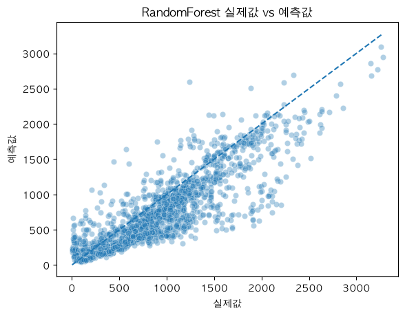
점선은 실제값과 예측값이 완전히 같은 경우를 나타낸다. 점이 점선에 가까울수록 예측이 정확하다. 그래프에서는 저·중간 대여량 구간에 점이 비교적 밀집하지만, 대여량이 큰 구간에서는 점선 주변으로 넓게 퍼진다. 즉, 피크 수요를 예측할 때 상대적으로 큰 오차가 발생할 수 있다.
8. 시간 흐름으로 실제값과 예측값 비교하기
테스트 데이터에 예측값을 추가하고, 앞부분 14일 분량의 시간별 행을 선 그래프로 비교한다.
prediction = best_model.predict(X_test)

compare_df = model_df.iloc[split_index:].copy()
compare_df["prediction"] = prediction

sample_compare = compare_df.head(24 * 14)

plt.figure(figsize=(16, 5))
sns.lineplot(
    data=sample_compare,
    x="Date",
    y="Rented Bike Count",
    label="Actual",
)
sns.lineplot(
    data=sample_compare,
    x="Date",
    y="prediction",
    label="Prediction",
)
plt.title("테스트 기간 일부: 실제 대여량 vs 예측 대여량")
plt.xticks(rotation=30)
plt.show()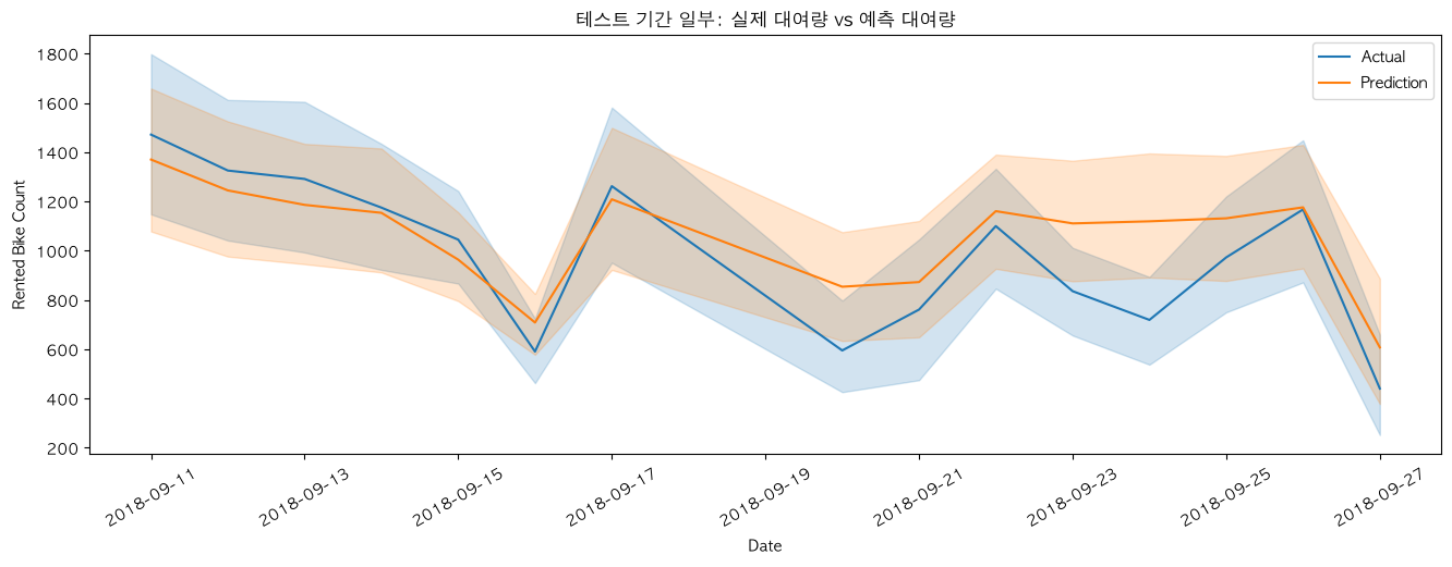
선 그래프는 날짜별 평균을 보여준다. 시간별 급격한 변화를 보려면 x축을 Date와 Hour를 합친 시각으로 바꾸는 방식도 활용할 수 있다. 이 그래프에서는 추세를 함께 따라가는지, 특정 날짜에 지속적으로 과대·과소 예측하는지를 확인한다.
9. 피처 중요도 확인하기
트리 기반 모델은 분할 과정에서 오차를 줄이는 데 기여한 정도를 feature_importances_로 제공한다. 원-핫 인코딩된 범주형 피처는 여러 컬럼으로 바뀌므로, 전처리 뒤의 피처 이름을 다시 가져와야 한다.
def get_feature_names(preprocessor):
    names = []

    for name, transformer, columns in preprocessor.transformers_:
        if name == "remainder" and transformer == "drop":
            continue

        if (
            hasattr(transformer, "named_steps")
            and "onehot" in transformer.named_steps
        ):
            onehot = transformer.named_steps["onehot"]
            names.extend(onehot.get_feature_names_out(columns))
        else:
            names.extend(columns)

    return np.array(names)


preprocessor = best_model.named_steps["preprocess"]
feature_names = get_feature_names(preprocessor)
importances = best_model.named_steps["model"].feature_importances_

importance_df = pd.DataFrame(
    {"feature": feature_names, "importance": importances}
).sort_values("importance", ascending=False)

print(importance_df.head(10))| 순위 | 피처 | 중요도 |
|---|---|---|
| 1 | Temperature | 0.3887 |
| 2 | Hour | 0.2300 |
| 3 | Solar Radiation | 0.0790 |
| 4 | Humidity | 0.0587 |
| 5 | Rainfall | 0.0565 |
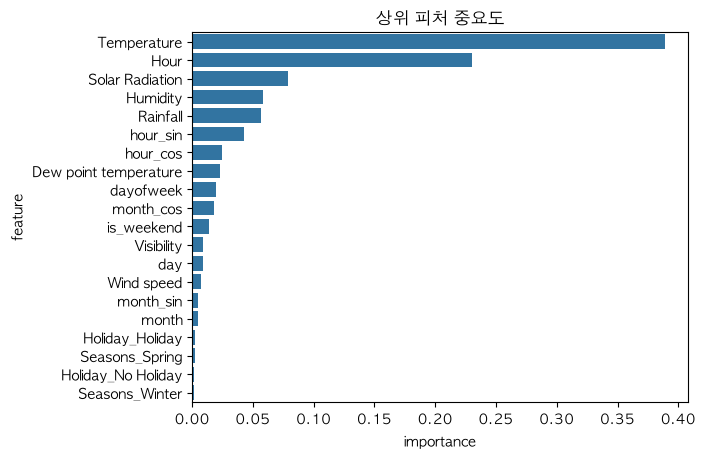
피처 중요도는 모델 내부에서의 상대적인 기여도다. Temperature의 중요도가 높다고 해서 기온만 바꾸면 대여량이 반드시 변한다는 인과관계를 뜻하지는 않는다. 서로 강하게 관련된 피처는 중요도가 나뉘거나 한쪽 피처에 몰릴 수 있다.
10. 튜닝된 결정트리 구조 시각화
plot_tree()로 튜닝된 결정트리의 상위 분기 구조를 확인할 수 있다. 전체 트리를 모두 그리면 너무 복잡해지므로 max_depth=4로 상위 구조만 표시한다.
from sklearn.tree import plot_tree

tree_model = dt_grid.best_estimator_.named_steps["model"]
feature_names = get_feature_names(
    dt_grid.best_estimator_.named_steps["preprocess"]
)

plt.figure(figsize=(24, 10))
plot_tree(
    tree_model,
    max_depth=4,
    feature_names=feature_names,
    filled=True,
    fontsize=9,
)
plt.title("튜닝된 결정트리 상위 구조")
plt.show()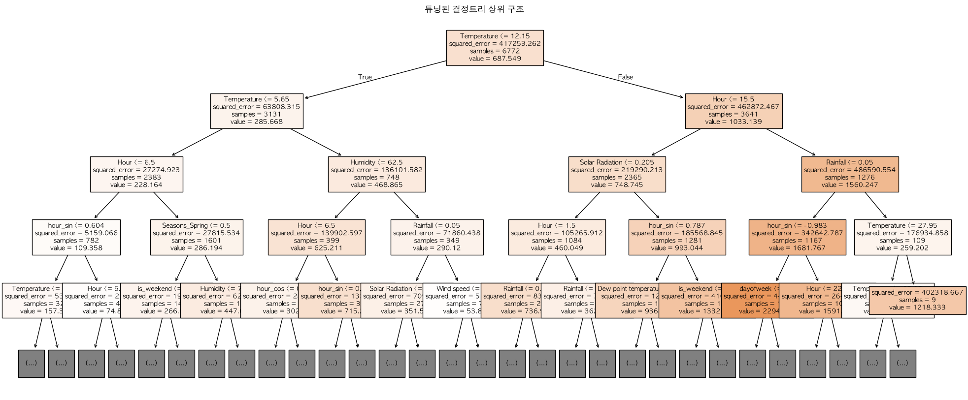
회귀 트리의 각 노드에는 분할 조건, 해당 노드의 MSE, 샘플 수, 예측 평균값이 표시된다. filled=True는 예측값 크기에 따라 노드 색을 다르게 표시해 높은 수요와 낮은 수요 구간을 구분하기 쉽게 만든다.
11. 핵심 정리
- 평균만 예측하는 Dummy 모델을 기준선으로 두고 여러 회귀 모델을 비교해야 성능을 판단할 수 있다.
- 이번 테스트 구간에서는 RandomForest가 RMSE
341.58, R20.6752로 가장 좋은 결과를 보였다. - 결정트리는 비선형 관계를 학습할 수 있지만 과적합하기 쉬우므로 깊이와 리프의 최소 샘플 수를 조절해야 한다.
- 교차 검증에서 선택된 하이퍼파라미터가 특정 테스트 기간에서도 항상 최고 성능을 보장하지는 않는다.
- 산점도는 예측 오차가 어느 수요 구간에서 커지는지 보여주고, 시간 흐름 그래프는 날짜별 추세를 함께 따라가는지 보여준다.
- 피처 중요도는 모델의 분할 기여도이지 인과관계가 아니다.