Chapter 8. Gaussian filtering and smoothing

Introduction

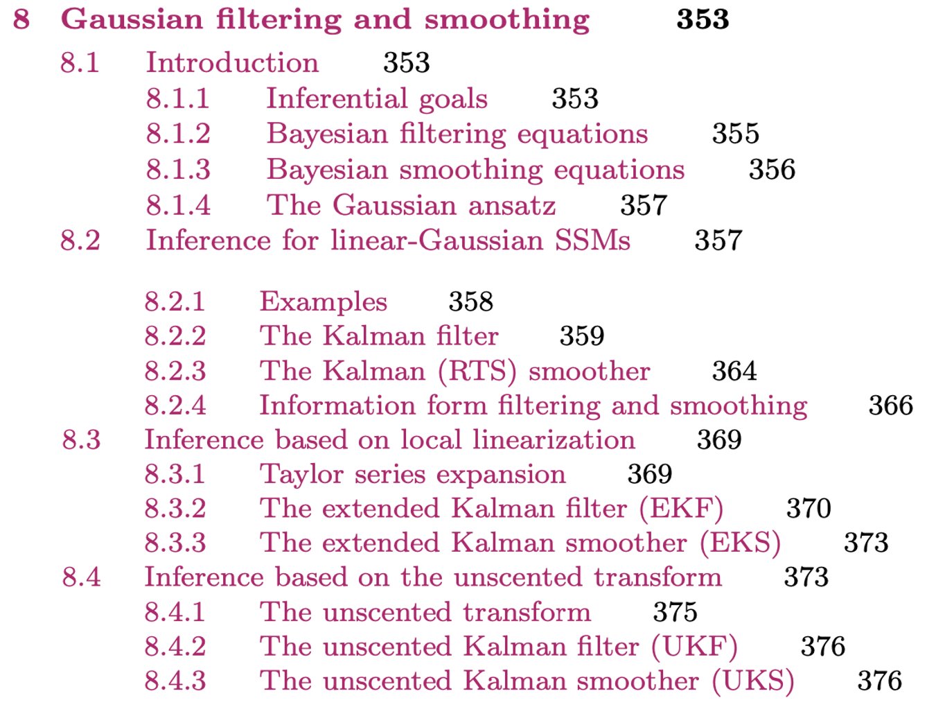
Probabilistic Machine Learning 의 Chapter 8 인 Gaussian filtering and smoothing 에 대해 정리하고자 한다. 이번 포스트에는 8.4 Inference based on the unscented transform 까지의 내용을 다루고 있다.

https://probml.github.io/pml-book/book1.html

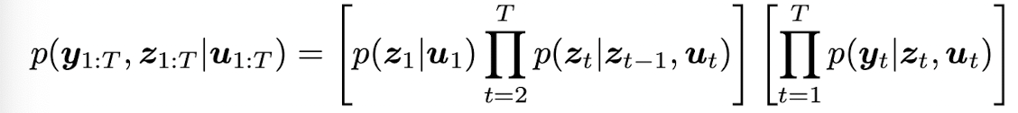
$z_t$ 는 hidden variables at time t, $y_t$ 는 실제 observations, $u_t$
는 optinal inputs 이다. term $p(z_t|z_{t-1},u_t)$ 는 transition model, $p(y_t|z_t, u_t)$는 observation model 이라 부른다.

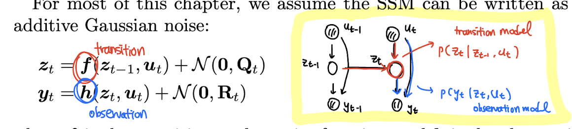
위와 같은 graphical model 로 간단하게 나타낼 수 있다. SSM 에 대한 더 세부적인 내용은 더 있지만, 우선은 위와 같은 chain-structured graphical model 처럼 conditional independencies 를 가진 latent variable sequence models 라고 생각해볼 수 있다.

Inferential goals

sequence of observation 과 known model 이 있을 때, SSM 의 main task 중 하나는 "hidden state" 에 대한 posterior inference 를 전개하는 것이다. 이는 "state estimation" 이라 부른다.

예를 들어 2d 공간에서 시간 t 에 대해 비행기가 두 차원의 위치와 속도 정보 $z_t$ 를 가지고 있다고 하자. 이 때 카메라의 문제 등 기술적 한계로 비행기의 t 시간까지의 noisy 한 위치 $y_{1:t}$ 만 (속도는 관측불가) 관찰가능하다고 할 때, 우리는 이 데이터를 기반으로 위치와 속도 정보를 추정하고자 하는 것이다.

즉 belief state $p(z_t|y_{1:t})$ 를 계산하기 위해 어떠한 모델을 쓸 것이고, 우리는 이것을 Bayesian filtering 부른다. 특히 Gaussian 을 이용해 belief state 를 추정할 때 우리는 "Kalman filter" 를 사용하여 이 문제를 풀 수 있다.

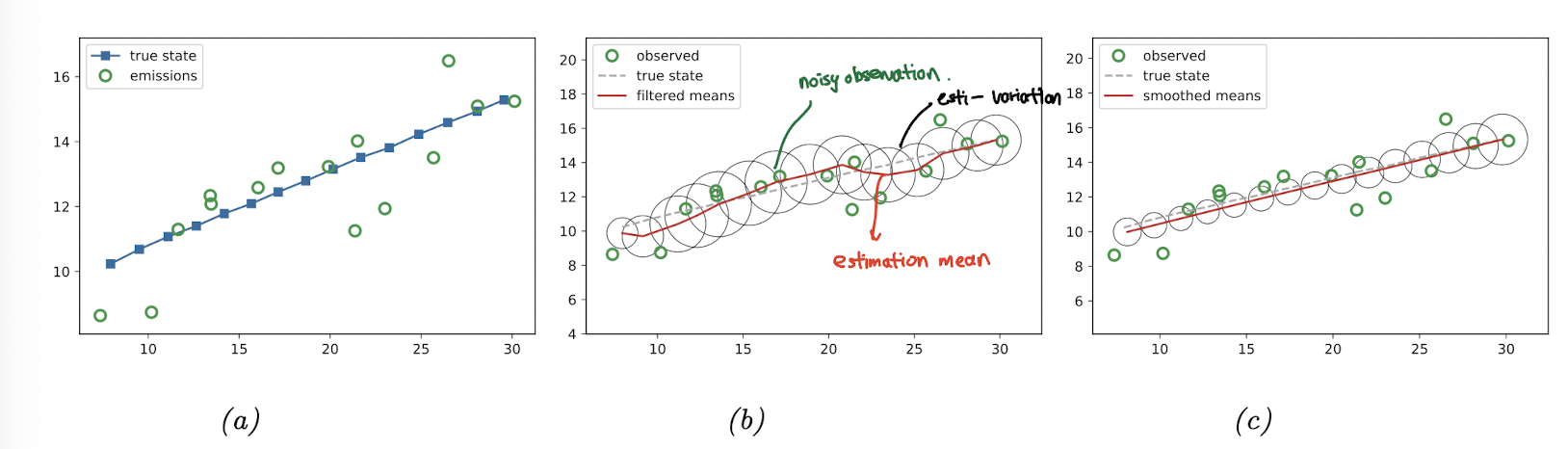
(a) 처럼 true state 와 observation (emission) 이 있다고 할 때, Kalman filter 를 사용하면 (b) 에서처럼 hidden state 에 대한 estimation 을 구할 수 있다.

또 다른 task 는 smoothing problem 이다. 이는 $p(z_t|y_{1:T}$ 를 offline dataset 를 이용해 추정하는 task 이다. T 는 t 보다 더 뒤의 시간대이고, 이미 있는 여러 시간대의 데이터를 이용해 좀 더 state estimation 을 narrow down 하는 과정이라고 생각할 수 있겠다. 이 또한 Kalman smoother 이라 부르고 추후에 다룰 것이다.

Bayesian filtering equations

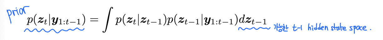
Bayes filter 는 주어진 이전 스텝의 prior belief $p(z_{t-1}|y_{1:t-1}$ 과 새로운 observation $y_t$ 를 기반으로 belief state $p(z_t|y_{1:t}$ 를 recursive 하게 계산하는 알고리즘이다. (online)

prediction step 은 우리가 아는 Chapman-Kolmogorov equation 의 형태이고, update step 도 Bayes' rules 를 이용한다.

Bayesian smoothing equations

offline setting 에서 smoothing 은 $p(z_t|y_{1:T}$ 을 계산하는 것이다. 이는 filtering pass 를 통해 T 까지 쭉 계산하고, 다시 t까지 backward 움직이는 방식을 사용하고 이를 forwards filtering backwards smoothing (FFBS) 라고 부른다.

Inference for linear-Gaussian SSMs

가장 기본이 되는 형태인 linear Gaussian state space model (LG-SSM) 에 대해 먼저 설명하고 있다. (linear + Gaussian) 근본

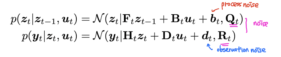
이는 아까 그렸던 graphical model 과 같은 기호를 사용하고 있다. $F_t$ 와 $H_t$ 가 곱해지고 noise 가 더해짐으로써 transition model 과 observation model 이 정의된다.

The Kalman filter

Kalman filter (KF) 는 Bayesian filtering for linear Gaussian state space model 알고리즘 그 자체이다. notation 이 굉장히 많기 때문에 잘 짚고 넘어가야 한다.

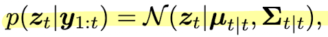
이는 belief state 이고 이와 더불어, $y_{1:t'}$ 의 posterior mean, covariance 를 $\mu_{t|t'}$, $\Sigma_{t|t'}$ 라고 지칭한다. 알고리즘의 derivation 전에 먼저 알고리즘이 어떻게 동작하는지를 먼저 설명하고 두 가지 방식의 derivation 을 기술하도록 하겠다.

Predict step

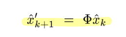
한 시점 뒤에 있는 hidden state 의 prediction 을 time update step 이라 부른다. 이는 다음과 같이 정의된다.

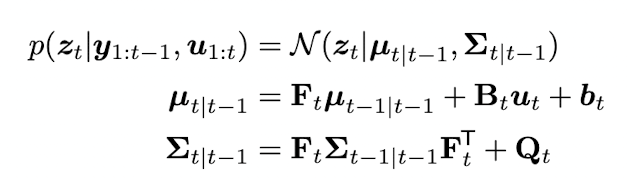
optional input 과 y 에 대한 t-1까지의 observation 을 이용해 hidden state $z_t$ 를 Gaussian 으로 표현한다. 아직 $y_t$ observation 정보는 사용되지 않았고, prior 정보만 사용되고 있다.

Update step

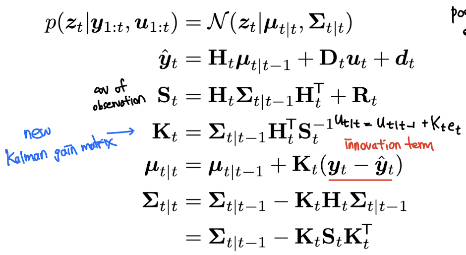
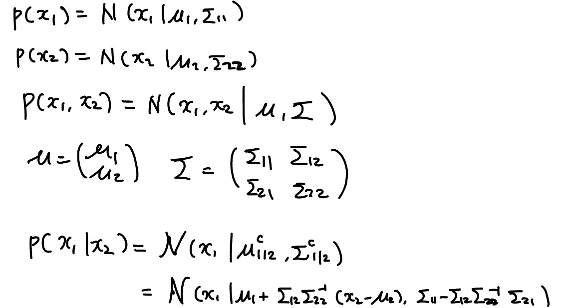
update step 에는 $y_t$ observation 을 활용해 hidden state 를 update 한다. 이는 다음과 같이 표현된다.

$K_t$ 는 Kalman gain matrix 이고, $\hat{y_t}$ 는 expected observation 이며, $\mu_{t|t}$ 에서 $K_t$ 옆에 곱해져 있는 $y_t - \hat{y_t}$ 는 residual error (또는 innovation term) 이라 부른다.

다음 식을 보다 더 직관적으로 이해해보자. $\mu_{t|t}$ 는 $\mu_{t|t-1}$ 에 Kalman gain matrix 와 error signal $e_t$ 를 곱해줘서 더해준 것이다. 이 때 $K_t$ 를 자세히 보면 만약 $H_t$ 가 identity matrix 일 때 $K_t = \Sigma_{t|t-1}S_t^{-1}$ 으로, inverse signal to noise ratio 라고 생각할 수 있다. 즉 우리가 강한 prior 또는 강한 noise 가 있다면, $|K_t|$의 크기는 작아질 것이고, prior 가 약하다면 크기가 커질 것이기 대문에 좀 더 correction term 에 힘을 줄 수 있는 것이다.

Posterior predictive

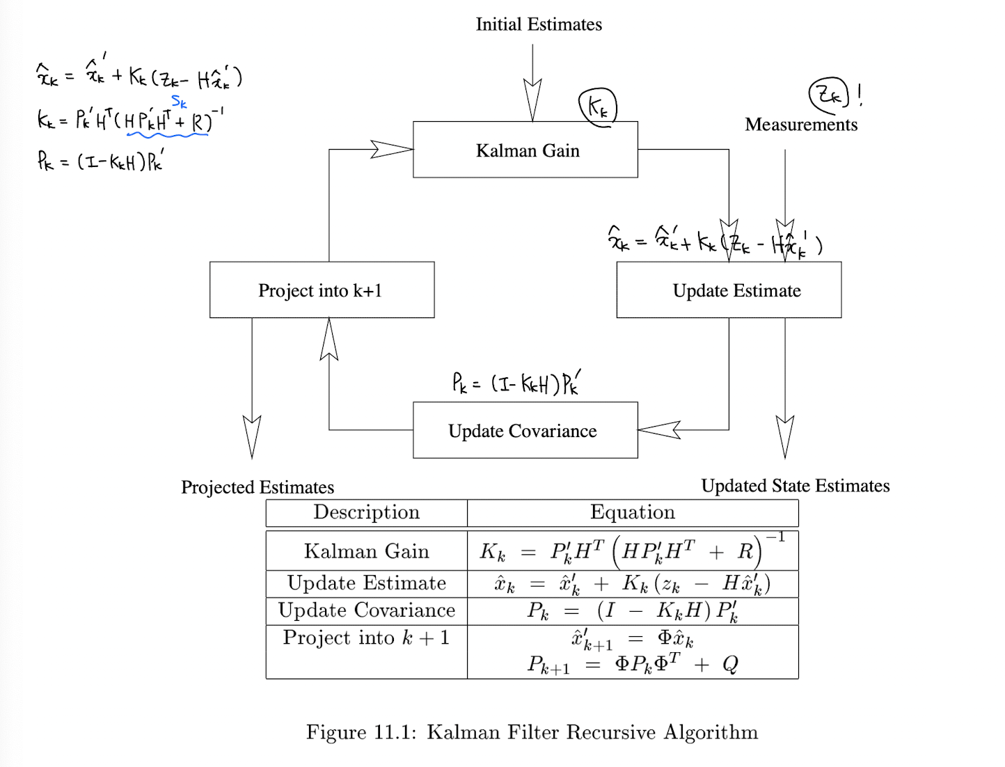
여태 matrix form 으로 살펴보았는데 이를 Bayesian framework 에서 좀 더 자세히 보도록 하자. one-step-ahead posterior predictive density for the observations 을 계산하기 전에 observation $y_t$ 를 사용하지 않고 먼저 latent states 의 one-step-ahead predictive density 를 계산해보자.

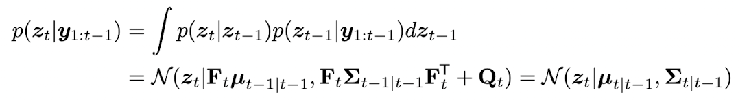
이 $z_t$ 를 marginalize out 해서 prediction about observation 으로 바꿔보면 다음과 같다.

이는 observation 의 log-likelihood 를 계산할 때도 사용되는데, new posterior 를 계산할 때의 normalization constant 는 다음과 같이 계산할 수 있다.

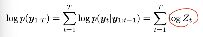
이는 결국 sum of the log probabilities of the one-step-ahead measurement predictions 이다. 그리고 이는 각 step 에서 model 이 얼마나 측정값에 대해 놀랐는지에 대한 정보량에 대한 값이기도 하다. 이 깜놀의 양을 상대적인 hidden state 에 대해 분배해서 posterior 이 되는 것이다.

We can generalize the prediction step to predict observations K steps into the future by first forecasting K steps in latent space, and then "grounding" the final state into predicted observations.

이는 바로 generating observations at each step in order to update future hidden states 의 동작을 가진 RNN 과 대비된다고 언급하고 있다.

Derivation (Murphy book version)

먼저 murphy 에서 그대로 소개하고 있는 유도 과정을 따라가 보도록 하자.

먼저 prediction setp 을 유도할 것이다. Joint predictive distribution for states 는 다음과 같이 표현할 수 있다.

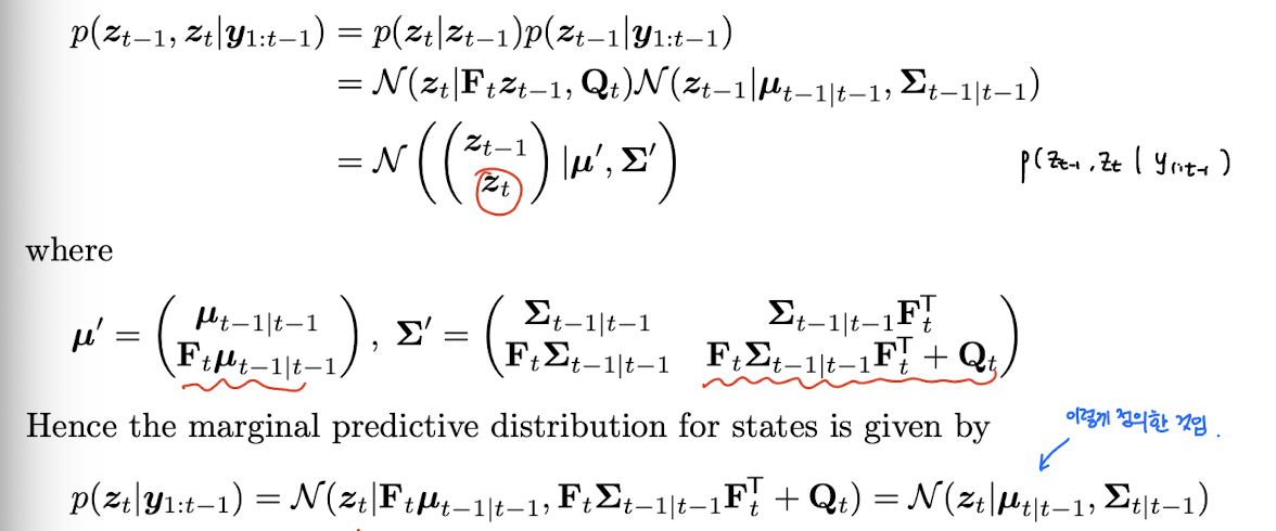
이후 observation $y_t$ 정보를 update 하는 measurement update step 이다. joint distribution for state and observation 은 다음과 같이 표현할 수 있다.

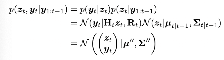
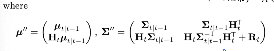
여기서 다음 step 과정이 사실 좀 intuition 에 의하기 보다는 공식에 의해서 나오는데 우선 다음 식을 보자.

이는 joint 식을 conditional 로 전환하는 공식인데 위 공식을 이용해서 observation 을 update 하면 우리가 아는 그 Kalman filter 식이 나온다.

Derivation (Tony Lacey version)

위의 derivation 이외에 다른 관점에서 derive 한 내용이 있어서 소개하고자 한다.

https://web.mit.edu/kirtley/kirtley/binlustuff/literature/control/Kalman%20filter.pdf

여기선 notation 이 조금 다르다.

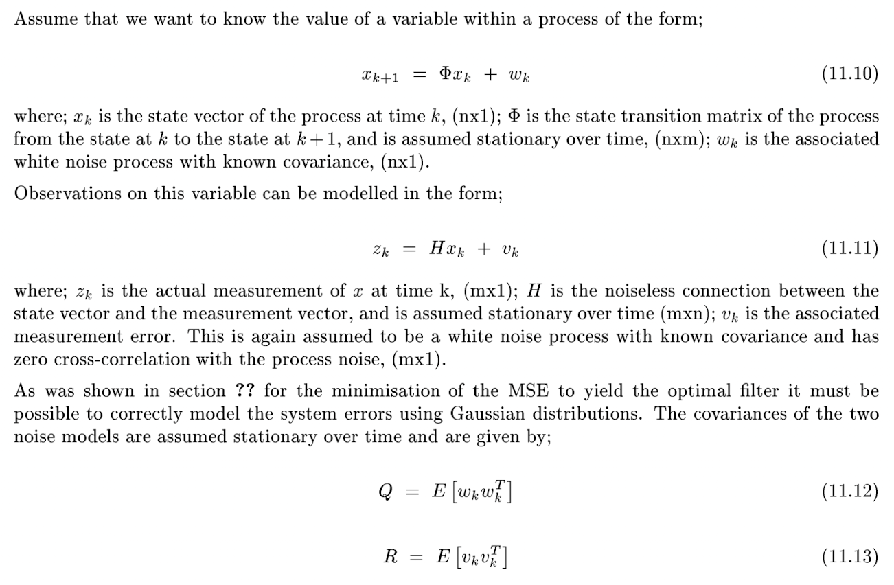
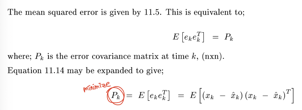
$x_k$ 가 state vector, transition matrix는 $\Phi$, measurement 는 $z_k$, observation matrix 는 $H$ 이다. MSE 를 최소화하는 optimal filter 하기 위해 먼저 system error 를 Gaussian 을 이용해 정의한다.

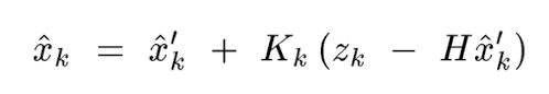
기존 system knowledge 로부터 계산가능한 $\hat{x}_k$ 의 prior estimate 를 $\hat{x}'_k$ 라고 하자. 이 old estimate 와 measurement data 를 이용해서 new estimate 를 만드는 update equation 을 다음과 같이 쓸 수 있다.

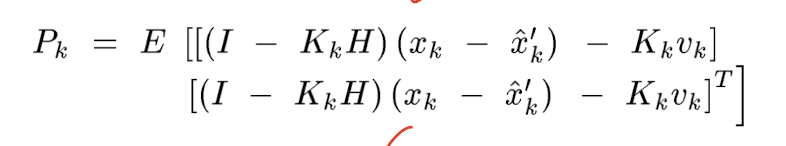
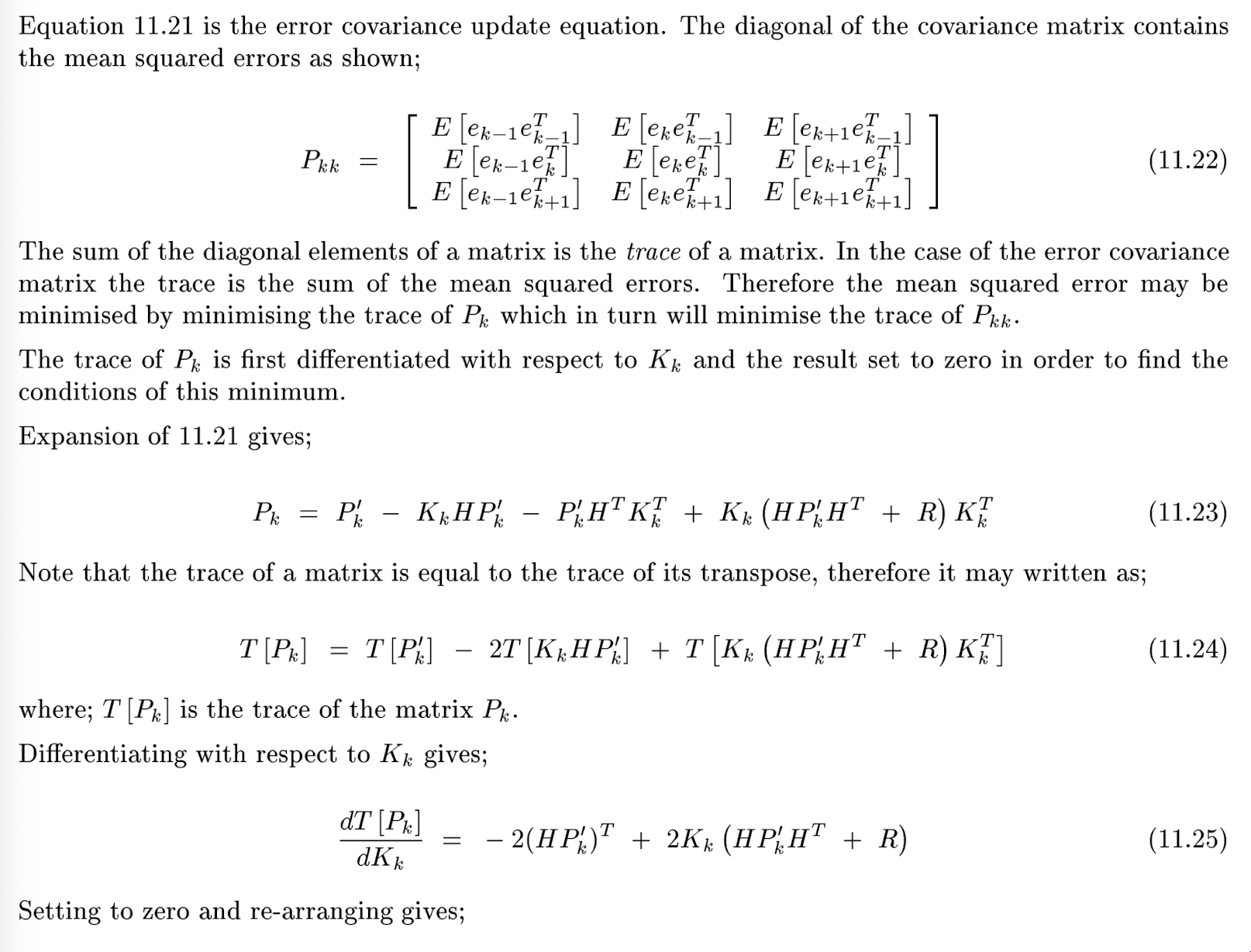
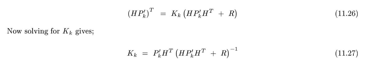
(중요) 우리는 아직 Kalman gain $K_k$ 가 어떻게 생겼는지 모른다. 아래에서 $P_k$ 를 최소화하는, 즉 system error 를 최소화하는 Kalman gain 이 어떻게 생겼는지를 유도한다.

이 때 observation $z_k$ 대신에 $Hx_k + v_k$ 를 대입하고 이를 정리하면 $P_k$ 는 다음과 같이 정리할 수 있다.

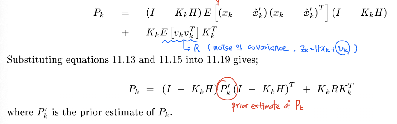
주의해서 보아야 할 점은, $P_k$ 의 정의는 $x_k - \hat{x}_k$ 이고 $P_k'$ 의 정의는 $x_k - \hat{x}_k'$ 즉 system knowledge 로부터 계산한 prior estimate 라는 점이다.

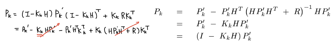
마지막으로 맨 처음에 사용했던 system knowledge 를 이용한 prior estimate of hidden stsate 를 구하면 하나의 스텝을 마무리할 수 있다.

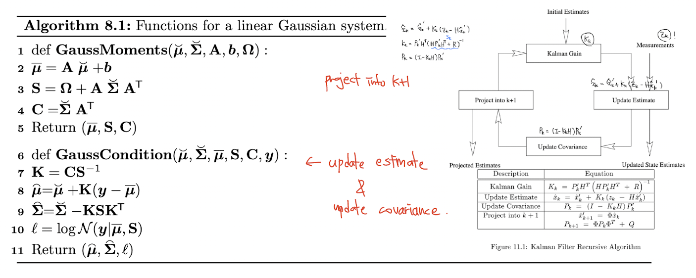
아래 그림은 전체적인 Kalman filter 의 알고리즘의 다이어그램이다.

Abstract formulation

다시 murphy 책으로 돌아와서, Kalman filter equation 을 더 깔끔하게 표현하고 있다.

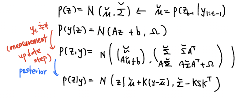
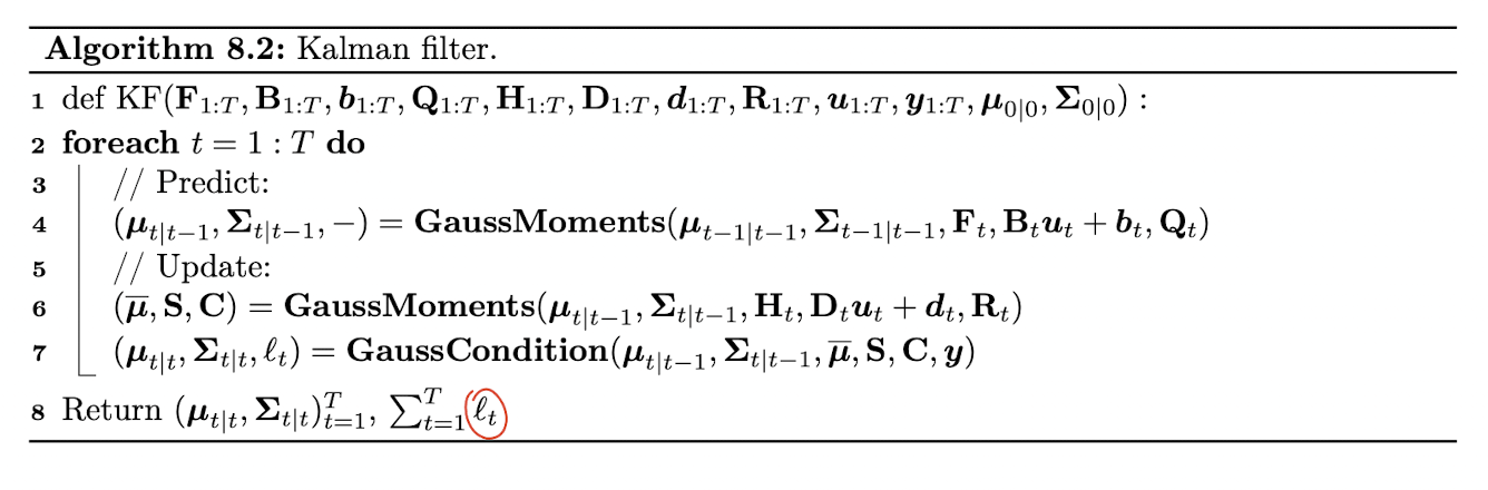
개인적으로 Kalman filter 를 가장 직관적으로 보여주는 연산은 Algorithm 8.1, GaussCondition line 8 이라 생각한다. 이전 스텝에서 구한 hidden state 정보를 통해 추정한 현재 y 의 추정치와의 error 에 Kalman gain 을 곱해서 현재 스텝에서의 hidden state 정보를 update 하고 있다.

The Kalman (RTS) smoother

앞선 설명에서는 각 time step t 마다 belief state $p(z_t|y_{1:t}$ 를 순차적으로 계산하는 Kalman filter 에 대해 다루었다. 이는 tracking 과 같은 online inference problem 에 적합하다. 하지만 offline setting 에서는 past/future data 를 활용하여 t 의 hidden state, 즉 $p(z_t|y_{1:T}$ 를 계산함으로써 uncertainty 를 더 줄일 수 있다.

RTS (Rauch-Tung-Striebel) smoother 라고도 불리우는 Kalman smoothing algorithm 은 linear-Gaussian 으로써 HMM forwards-filtering backwards-smoothing algorithm 과 매우 유사하다(고 한다).

Algorithm

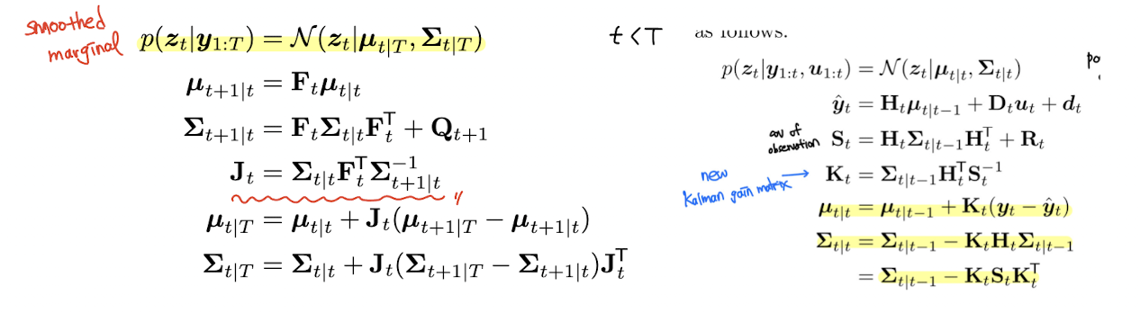
새로운 J 라는 matrix 가 등장한다. 또한 t|T 가 계산되는 과정에서 t+1|T 가 사용되고 있고, 앞서 Kalman filter 를 통해 구했던 t|t 도 계속 사용되는 것을 확인할 수 있다. 즉 이는 forward 과정으로 쭉쭉 T까지 filter 를 씌우며 계산을 한 뒤에, 다시 반대로 한 step 씩 backward 과정으로 smoothing 하는 알고리즘인 것이다.

Derivation

유도과정은 다음과 같다. Kalman filter 와 유도과정이 매우 유사하다. Joint distribution 을 구하고 이를 future state에 conditioning 한다.

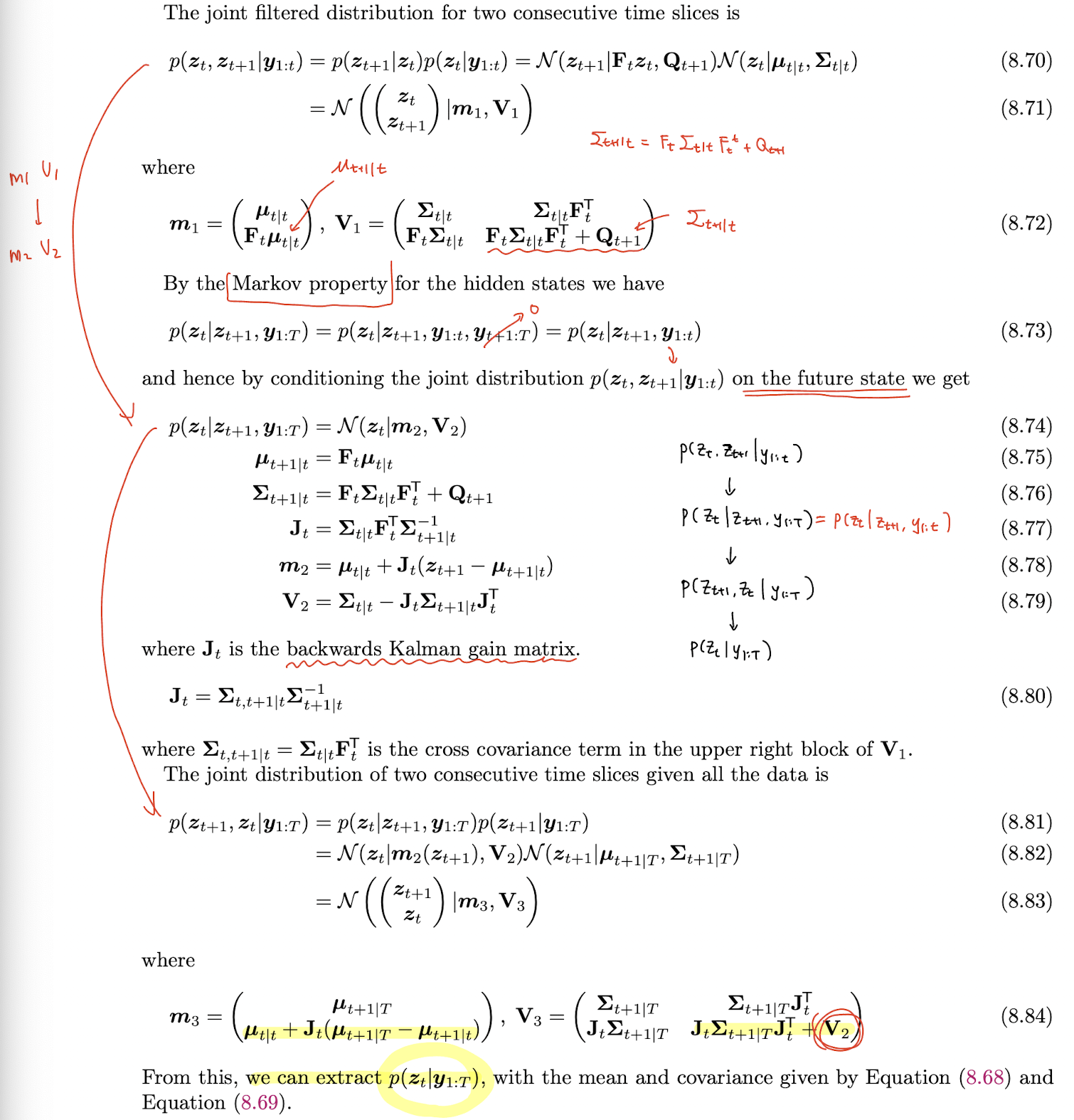
먼저 forward 과정에서 미리 구해두었던 정보들을 통해 t 와 t+1 time step 에서의 hidden state joint filtered distribution 을 구한다. (8.72) 그 뒤에 $z_{t+1}$ 에 condition 한 $z_t$ 의 값을 유도해내고, 이 과정에서 backwards Kalman gain matrix $J_t$ 가 등장한다. 마지막으로 이 conditional probability 로부터 $p(z_t|y_{1:T})$ 를 추출해낸다.

Inference based on local linearization

linear 한 dynamic system 및 observation 에서 사용되는 Kalman filter, smoother 를 알아보았다. 이를 확장하여 system dynamic 및 observation model 이 nonliear 한 경우에 대해서 어떻게 되는지를 알아보도록 하겠다.

가장 기본이 되는 아이디어는 소제목에서도 나와있듯이 local linearization 으로, first order Taylor series expansion 을 이용해서 stationary non-linear synamical system 을 non-stationary linear dynamical system 으로 근사한다. 이러한 접근을 extended Kalman filter (EKF) 라고 부른다.

Taylor series expansion

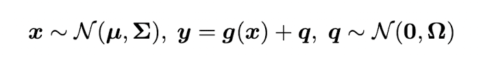
$x$ ~ $\mathcal{N}(\mu, \Sigma)$ 이고 함수 $y=g(x)$, where $g : \R^n$ ->$\R^m$ 는 미분 가능한 invertible 함수라 가정하자. 그렇다면 y 에 대한 Pdf 는 다음과 같이 계산할 수 있다.

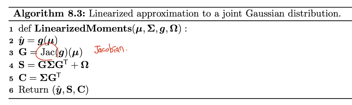
이는 intractable 하기 때문에 approximation 을 구해야 한다. $x = \mu + \delta$, where $\delta$ ~ $\mathcal{N}(0, \Sigma)$ 라 가정할 때, 우리는 다음과 같이 first order Taylor series expansion 을 쓸 수 있다.

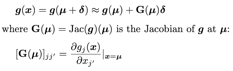
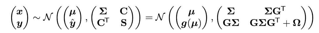
이를 이용해 계산한 y의 Mean 은 $g(\mu)$ 가 될 것이고, y의 covariance 는 $G(\mu) \,\Sigma\, {G(\mu)}^T$ 로 계산될 것이다.

이를 이용해 위와 같은 상황에서의 joint distribution p(x,y) 를 계산하면 다음과 같이 쓸 수 있다.

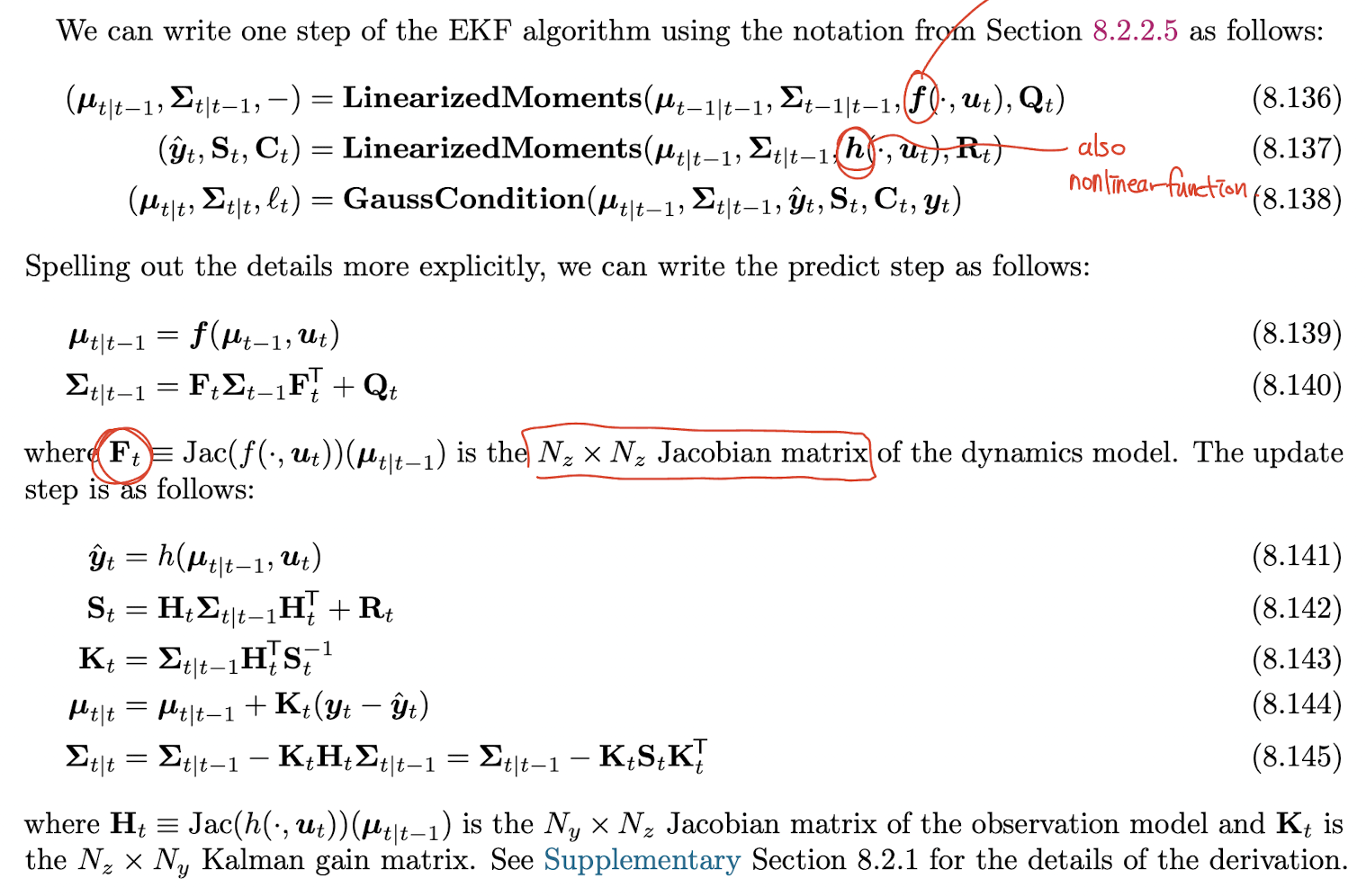
The extended Kalman filter (EKF)

위의 approximation 방식을 활용하여 extended Kalman filter 알고리즘을 살펴볼 것이다. 먼저 $\mu_{t-1|t-1}$ 을 중심으로 dynamic model 을 linearize 하고 one-step-ahead predictive distribution $p(z_t|y_{1:t-1},u_t)$ 를 계산하여 얻는다. 이후 $\mu_{t|t-1}$ 을 중심으로 observation model 을 linearize 하여 Gaussian mean & covariance update 수행함으로써 하나의 time step 에서의 belief state 를 계산할 수 있게 된다.

code implementation & example

최근 들어 많이 사용하고 있는 pyro repository 에도 구현된 EKF 내용이 있어 살펴 보고 직접 코드를 실행해보았다.

https://github.com/pyro-ppl/pyro/blob/dev/pyro/contrib/tracking/extended_kalman_filter.py

update 함수를 주로 보았는데 다음과 같이 구현되어 있다.

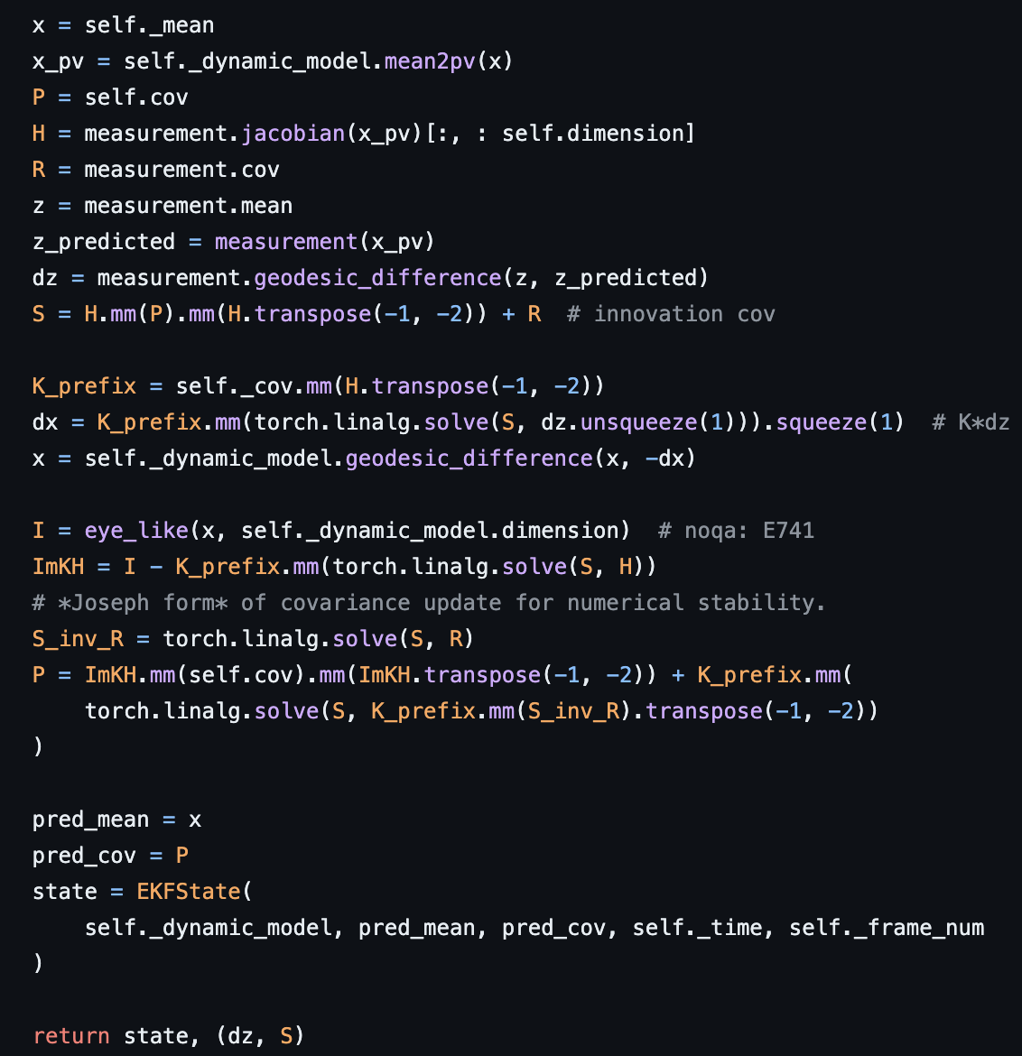
몇가지 notation 은 다르다. x 는 hidden state value 값이고 (pv 는 process variable 또는 position velocity.. 모르겠다 아무튼 vector 를 깔끔하게 정리하는 것 같다) P 는 cov term, H 는 measurement 의 jacobian 이고, z 는 관측값, z_predicted 는 state 정보를 이용한 추정 관측값이다. non-linear system 이기 때문에 Euclidean 보다 geodesic_difference 함수를 사용한 것으로 보인다. 알고리즘을 충실히 따라 EKFState 라는 class 를 반환하는 것으로 보이고, update & predict 함수를 통해 online learning 을 수행한다.

그 다음으로 ekf.ipynb 에서 주어진 샘플 코드를 조금 수정해 visuazation 해보았다.
https://github.com/pyro-ppl/pyro/blob/dev/tutorial/source/ekf.ipynb

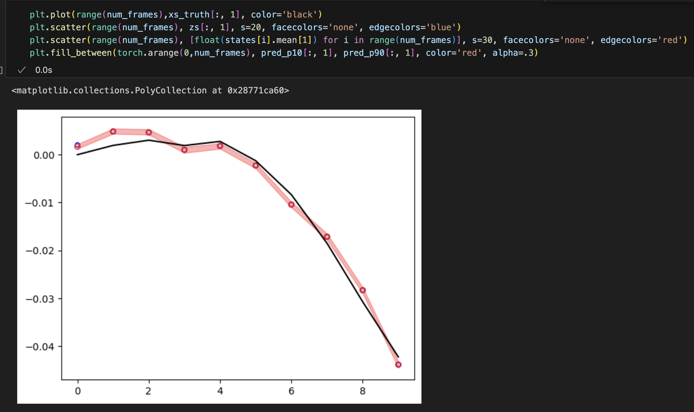
true state 가 검정색, 파란색이 관측값, 빨간색이 추정 state 의 평균값이다.

Accuracy

EKF 는 simplicity, efficiency 때문에 널리 이용된다. 하지만 잘 작동하지 않는 경우도 있다. 첫번째는 prior covariance 가 클 때이다. 이 경우 prior distribution 이 너무 광범위해서 probability mass 의 상당 부분을 우리가 관심 있는 부분인 $\mu_{t-1|t-1}$ 부분과 멀리 있는 곳에 보내야 한다. 다시 말해, EKF 는 선형화가 한 지점에서만 이루어지기 때문에 prior covariance 가 크면, 즉 state uncertainty 가 크다면 비선형 함수의 다양한 부분을 거쳐서 probability mass 값이 전달되어야 하는데 EKF 알고리즘 특성 상 local 하게 보기 대문에 실제 동작을 제대로 모델링 하지 못할 수 있다는 점이다. 또한 두번째로 nonlinearity 가 너무 크면 잘 작동하지 않을 수 있다.

좀 더 발전된 방법으로 second order EKF, Iterated EKF, unscented Kalman filter 를 소개하고 있다.

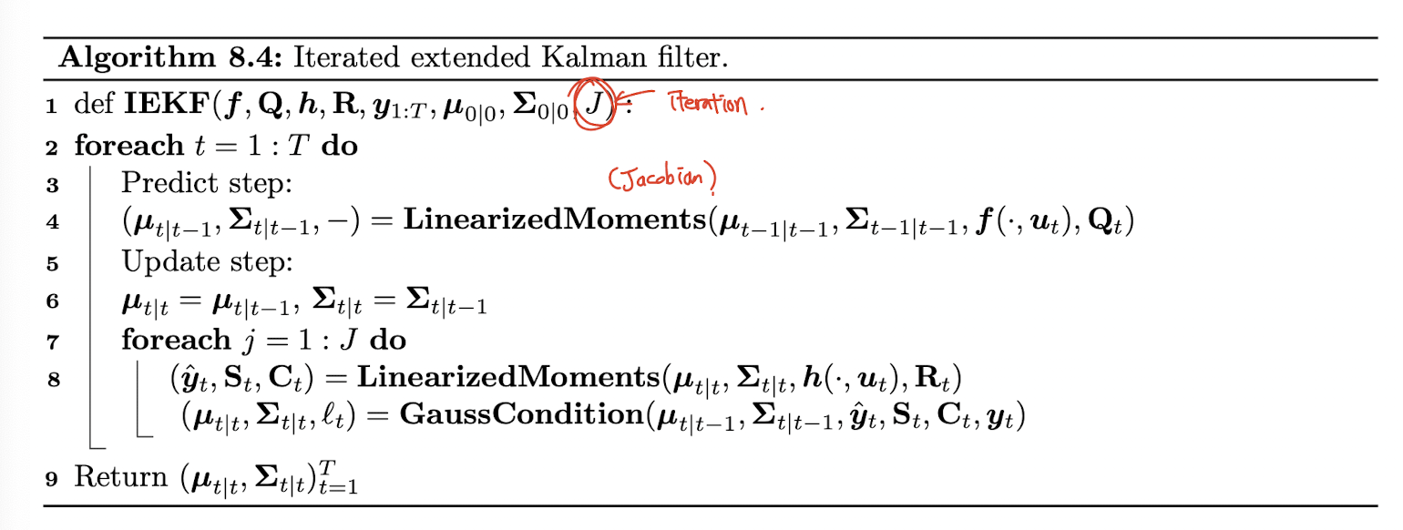
Iterated EKF

EKF 의 정확도를 높이기 위해 "observation model" 의 $\mu_{t-1|t-1}$ 근처가 아닌 current posterior $\mu_{t|t-1}$ 근처를 반복적으로 re-linearizing 하는 방법이 있다. https://arxiv.org/abs/2307.09237 이런 논문도 있었다.

Inference based on the unscented transform

전 섹션에서 taylor series expansion 을 이용한 local linearization 을 차용한 EKF 에 대해 알아보았다. 여기선 조금 다른 근사 방법을 사용하는 unscented Kalman filter (UKF) 에 대해 알아보고자 한다.

기본적인 아이디어는, dynamics 및 observation model 을 linearization 하고 Gaussian distribution 을 이 linear 된 model 에 pass 시키는 EKF 와 달리, joint distribution $p(z_{t-1}, z_t|y_{1:t-1})$ and $p(z_{t}, y_t|y_{1:t-1})$ 자체를 Gaussian 을 이용해 근사하고 numerical integration 을 통해 여러 moment 를 계산한 뒤에, 이 계산된 moment 를 이용해 marginal 및 conditional distribution 을 계산한다.

이러한 방식의 장점은, EKF 에 비해 더 정확하고 더 안정적이며, Jacobians 을 계산할 필요가 없기 때문에 non-differentiable model 에 대해서도 잘 작동한다는 점이다.

The unscented transform

다음 두 개의 random variable 이 있다고 가정해보자. $x$ ~ $\mathcal{N}(\mu, \Sigma)$ and $y=g(x)$, where $g : \R^n$ ->$\R^m$. unscented transform 은 p(y) 의 Gaussian approximation 을 구하기 위해 다음과 같은 방식을 사용한다.

1. 2n+1 sigma point, $\mathcal{X}_i$ 를 적절히 계산하고 그에 대응되는 weights $w_i^m$, $w_i^c$ 를 계산한다.

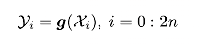
2. sigma point 를 nonlinear function 에 통과시켜 다음과 같은 2n+1 output 을 얻는다.
   

3. 이 set of points 로부터 moments 즉 mean, covariance 를 추정한다.

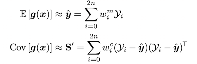
이러한 joint distribution 의 moment를 활용해서 앞선 EKF 와 같이 conditional probability 를 계산하고 이를 통해 계속 update 하는 방법이다.

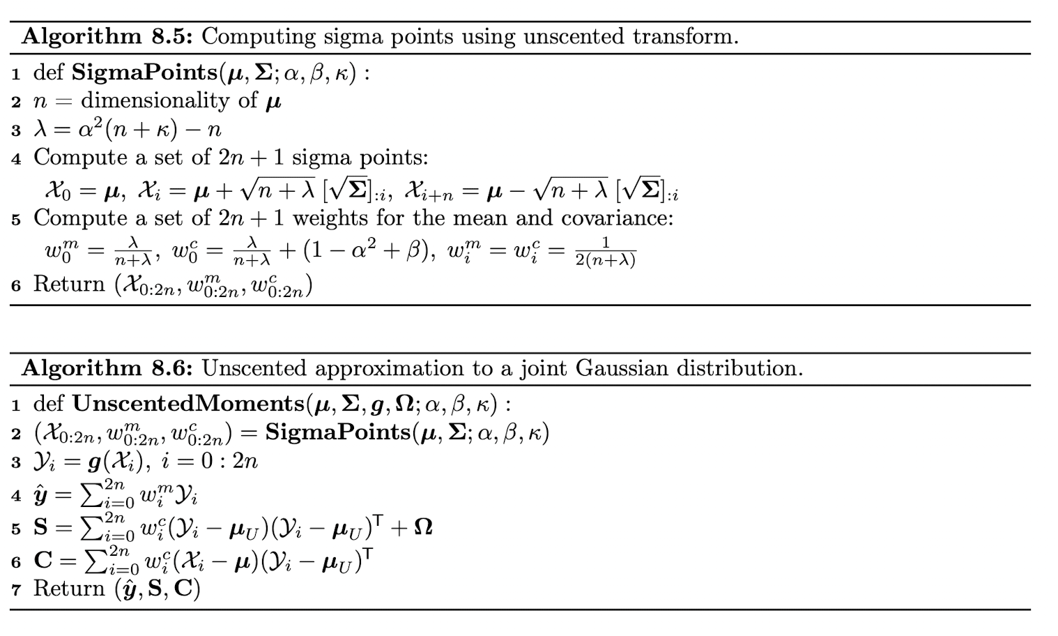
이 Sigma points 와 weight 는 alpha, beta, kappa 라는 hyperparameter 에 따라 달라진다. 일반적으로 많이 쓰이는 hyperparameter 가 존재한다.

The unscented Kalman filter (UKF)

unscented transform 을 두 번 사용한다. 한 번은 transition model 을 통과시켜 hidden state 값을 구할 때, 한 번은 observation model 을 통과시켜 estimated observation 값을 구할 때 사용되고, 마찬가지로 Kalman gain matrix 를 통해서 belief state 를 update 하게 된다.

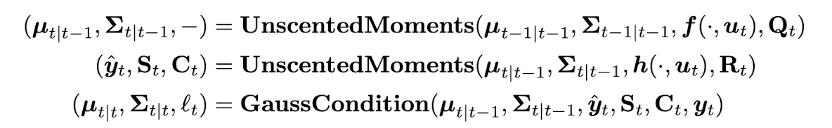
The unscented Kalman smoother (UKS)

unscented Kalman smoother (unscented RTS smoother) 또한 Kalman smoothing method 에서 nonlinearity 를 unscented transform 으로 근사하는 modification 이 들어간 방법이다. 이 때 reverse Kalman gain matrix $J_t$ 는 predicted covariance 와 cross covariance 로부터 얻어지는데 이 둘은 모두 unscented transform 에 의해 추정되는 값들이다.

특히 UK 정부는 이 unscented Kalman smoothing 방식을 COVID-19 contact tracing app 에도 사용했다고 한다. 사람들의 핸드폰의 bluetooth signal strength 시그널로부터 사람들 간의 distance 를 추정하고, 추정한 distance 와 다른 signal (duration, infectiousness level of the index case) 와 결합하여 risk of transmission 을 추정했다고 한다.