
Intro
최근 kaggle에서 굉장히 눈에 띄는 competition이 있었으니 바로, Predicting Molecular Properties라는 이름의 대회였다. 해당 competition은 브리스톨 대학교, 카디프 대학교, 임페리얼 칼리지 및 리즈 대학교로 이루어진 CHAMPS(CHemistry And Mathematics in Phase Space) 에 의해 주최되었으며, 수상하는 팀에게는 대학 연구 프로그램과 협력할 수 있는 기회가 주어진다고 한다.

예측 대상
우선 해당 대회의 도전과제는 소제목 및 Description을 통해 파악할 수 있다.
Can you measure the magnetic interactions between a pair of atoms?
In this competition, you will develop an algorithm that can predict the magnetic interaction between two atoms in a molecule
이번 대회를 통해 우리가 예측 해야 하는 것은 바로 분자 설계 시 한 쌍의 원자 간 결합으로 인해 발생하는 결합상수(Coupling Constant)를 예측하는 것이다.
결합 상수라는 것은 물리적 상호작용(여기서는 원자 간)의 세기를 나타내는 상수로서, 결합상수가 1일 때 완전결합이라고 한다. 아래에서 좀 더 자세히 살펴보겠지만, 제공되는 데이터에는 분자 및 원자에 대한 정보가 있으며 두 원자 간의 결합상수가 target value로 존재하고 있다.
학습 전략
처음 제공된 데이터를 보았을 때 train, test 외에 추가로 제공되는 데이터를 어떻게 활용해야 할지 난감했다. 그 이유는 structures 데이터를 제외하고는 모두 train 데이터에 대한 정보 밖에 없었기 떄문이다. 모델을 학습하고 예측할 때 당연히 train set과 test set의 차원의 크기가 같아야 했기 때문에 train에 대한 정보만 있는 데이터를 활용하는 것이 의미가 없다고 판단되었다. 그래서 최대한 활용할 수 있는 데이터만 사용하였으며 몇 가지 파생변수를 만들어 부족한 차원을 채워주었다.
모델 학습을 위해서는 LightGBM이라는 최근 캐글에서 가장 인기 있는 Gradient Boosting 기반의 모델을 사용하였다. 해당 데이터에는 type 이라는 분자의 타입을 구분하는 칼럼이 존재하는데, 처음 모델을 만들 때는 type 구분 없이 전체를 학습시켰으나 성능이 기대만큼 잘 나오지 않았다. 그래서 feature를 늘려야 하나 고민하던 중 우연히 Nanashi라는 사람의 kernel에서 전체 분자를 학습시키지 않고 분자의 type별로 따로 학습 및 예측을 진행하는 것을 보게 되었다. score를 보니 상당히 높은 score를 가지고 있었고 시도해볼 만 한 가치가 있다고 판단되어 이번 모델에 벤치마킹하여 적용하였다.
평가 방법
이번 대회에서는 Evaluation을 위해 평균절대오차(MAE, Mean Absolute Error)에 log값을 씌운 점수로 평가를 진행하게 된다. 공식 metric은 아래와 같으며, 완벽하게 예측했을 때 최종 점수는 -20.7232이다.
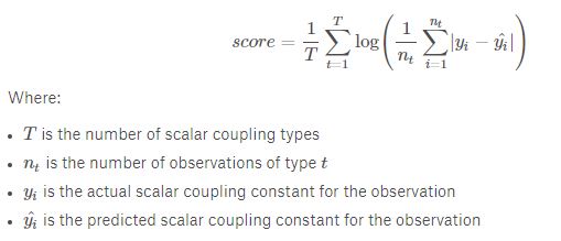
!코드 작성은 Jupyter lab을 이용하였으며, 아래 작성된 코드는 ipynb파일을 markdown으로 변환 후 업로드한 것이다.
import pandas as pd
import numpy as np
import os
import seaborn as sns
import matplotlib.pyplot as plt
from mpl_toolkits.mplot3d import Axes3D
from sklearn.model_selection import train_test_split
from sklearn.preprocessing import LabelEncoder
import lightgbm as lgb

# path
path_dir = 'C:/Users/USER/.kaggle/competitions/champs-scalar-coupling/'
file_list = os.listdir(path_dir)
file_list
['dipole_moments.csv',
'magnetic_shielding_tensors.csv',
'mulliken_charges.csv',
'potential_energy.csv',
'sample_submission.csv',
'scalar_coupling_contributions.csv',
'structures.csv',
'structures.zip',
'test.csv',
'train.csv']
1. Load Train/Test Data
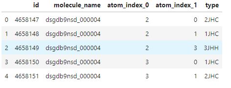
Columns
- molecule_name : 분자 이름
- atom_index_0 / atom_index_1 : 원자 인덱스
- type
- Coupling Constant(결합상수) : 물리적 상호작용(여기서는 원자 간)의 세기를 나타내는 상수, 결합상수가 1일때 완전결합이라고 함
train_df = pd.read_csv(path_dir+'train.csv')
test_df = pd.read_csv(path_dir+'test.csv')   # target = 'scalar_coupling_constant'

print('Length of train set: {}'.format(len(train_df)))
print('Length of test set: {}'.format(len(test_df)))
Length of train set: 4658147
Length of test set: 2505542
print('Unique molecule of train set: {}'.format(len(train_df['molecule_name'].unique())))
train_df.head()
Unique molecule of train set: 85003
print('Unique molecule of test set: {}'.format(len(test_df['molecule_name'].unique())))
test_df.head()
Unique molecule of test set: 45772
2. EDA
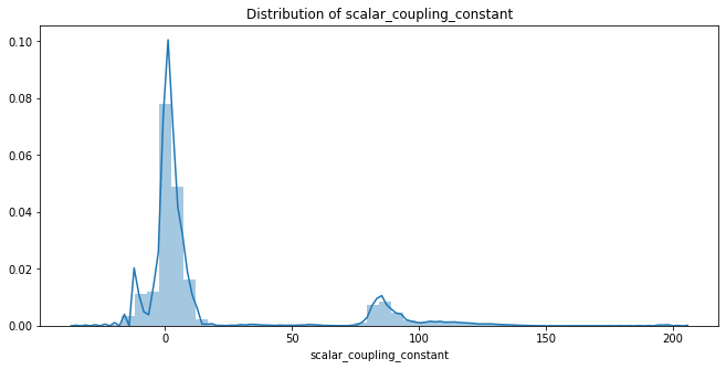
2.1 Distribution of Target ('scalar_coupling_constant')
- Min Value : -36.2186
- Max Value : 204.88
- 대부분이 -20 ~ +20 사이에 존재
- 작은 분포로 80 ~ 100 사이에 존재
# Distribution of target
print('Min Value of Target : {}'.format(train_df['scalar_coupling_constant'].min()))
print('Max Value of Target : {}'.format(train_df['scalar_coupling_constant'].max()))

plt.figure(figsize=(11, 5))
sns.distplot(train_df['scalar_coupling_constant'])
plt.title('Distribution of scalar_coupling_constant')
plt.show()
Min Value of Target : -36.2186
Max Value of Target : 204.88
2.2 Distribution of 'scalar_coupling_constant' by type
- '1JHC' type이 상대적으로 높은 scalar coupling 범위에 분포(+66.6 ~ +204.8)
- '2JHH' type이 상대적으로 낮은 scalar coupling 범위에 분포(-35.1 ~ +11.8
# Distribution of 'scalar_coupling_constant' by type
plt.figure(figsize=(14, 13))
for i, t in enumerate(train_df['type'].unique()):
    plt.subplot(4,2, i+1)
    sns.distplot(train_df[train_df['type'] == t]['scalar_coupling_constant'])
    plt.title('Distribution of coupling constant by type '+ t)
    plt.tight_layout()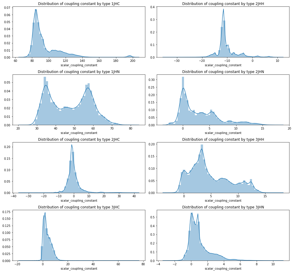
2.3 Count by 'type'
- 3JHC, 2JHC, 1JHC, 3JHH, 2JHH, 3JHN, 2JHN, 1JHN 순서로 높음
# Count by 'type'
type_index = train_df['type'].value_counts().index
type_cnt = train_df['type'].value_counts()

plt.figure(figsize=(11, 4))
sns.barplot(x=type_index, y=type_cnt)
plt.xlabel('type'); plt.ylabel('Count')
plt.title('Count by type')
plt.tight_layout()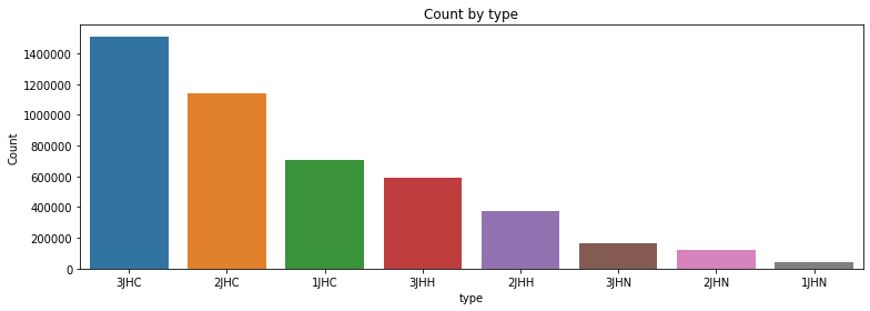
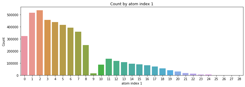
2.4 Count by atom index 0, 1
- atom index 0의 경우 9 ~ 18번이 가장 많이 분포
- atom index 1의 경우 1 ~ 8번이 가장 많이 분포
# Count by atom index 0, 1
for i in [0, 1]:
    atom_index = train_df['atom_index_'+str(i)].value_counts().index
    atom_cnt = train_df['atom_index_'+str(i)].value_counts()

    plt.figure(figsize=(11, 4))
    sns.barplot(x=atom_index, y=atom_cnt)
    plt.xlabel('atom index '+str(i)); plt.ylabel('Count')
    plt.title('Count by atom index '+str(i))
    plt.tight_layout()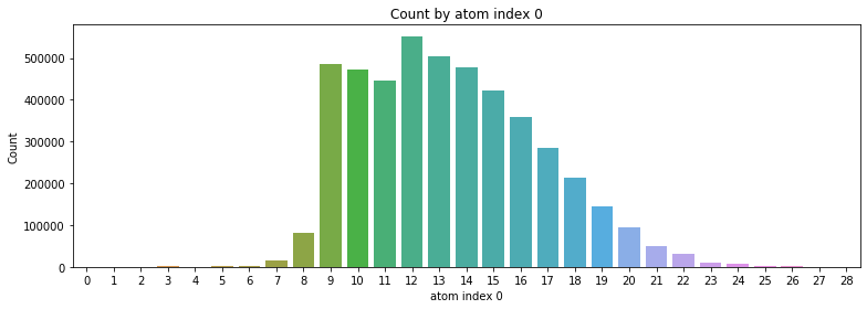
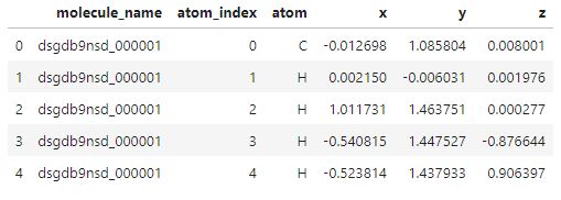
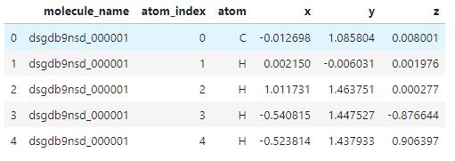
3. Load Structures Data
Columns
- molecule_name
- atom_index
- atom
- x, y, z axis of atom
structures_df = pd.read_csv(path_dir+'structures.csv')

print('Length of test set: {}'.format(len(structures_df)))
structures_df.head()
Length of test set: 2358657
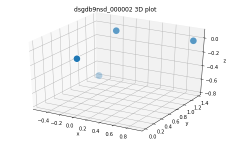
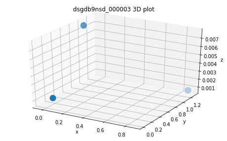
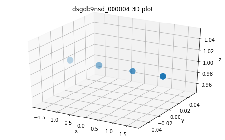
3.1. 3Dimension plot by Molecule
for name in structures_df['molecule_name'].unique()[:4]:
    structures_molecule =structures_df[structures_df['molecule_name'] == name]

    fig = plt.figure(figsize=(8, 5))
    ax = fig.add_subplot(111, projection='3d')
    ax.scatter(structures_molecule['x'], structures_molecule['y'], structures_molecule['z'], s=200, edgecolors='white')
    ax.set_title(str(name)+ ' 3D plot')
    ax.set_xlabel('x')
    ax.set_ylabel('y')
    ax.set_zlabel('z')
    plt.show()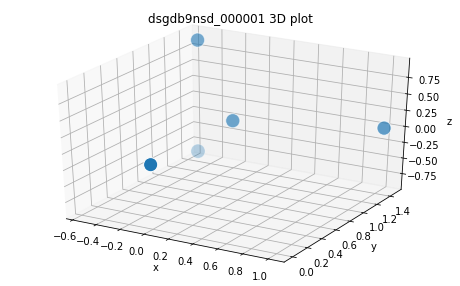
4. Preprocessing
4.1. Merge Train&Test - Structures Data
def mapping_atom_index(df, atom_idx):
    atom_idx = str(atom_idx)
    df = pd.merge(df, structures_df,
                  left_on  = ['molecule_name', 'atom_index_'+atom_idx],
                  right_on = ['molecule_name',  'atom_index'],
                 how = 'left')

    df = df.drop('atom_index', axis=1)
    df = df.rename(columns={'atom': 'atom_'+atom_idx,
                            'x': 'x_'+atom_idx,
                            'y': 'y_'+atom_idx,
                            'z': 'z_'+atom_idx})
    return df
train_merge = mapping_atom_index(train_df, 0)
train_merge = mapping_atom_index(train_merge, 1)
test_merge = mapping_atom_index(test_df, 0)
test_merge = mapping_atom_index(test_merge, 1)train_tmp = train_merge[['id','molecule_name','type']]
test_tmp = test_merge[['id','molecule_name','type']]
train_merge.head()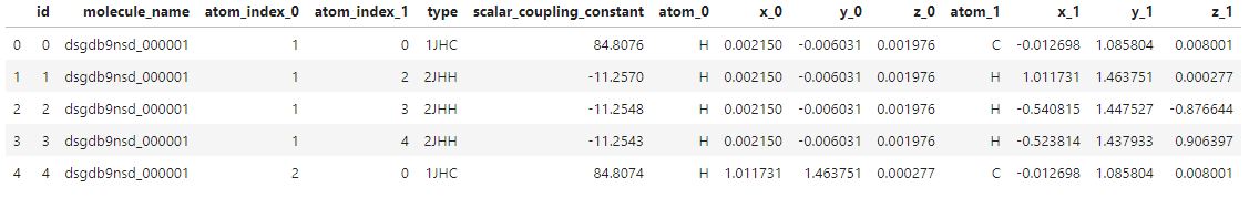
4.2. Derived variables - 'Distance'
- distance between x axis of atom index
- distance between y axis of atom index
- distance between z axis of atom index
- distance between atom
def dist_between_atom(df):
    # distance between axis of atom
    df['x_dist'] = (df['x_0'] - df['x_1'])**2
    df['y_dist'] = (df['y_0'] - df['y_1'])**2
    df['z_dist'] = (df['z_0'] - df['z_1'])**2

    # distance between atom
    df['atom_dist'] = (df['x_dist']+df['y_dist']+df['z_dist'])**0.5

    return df

train_dist = dist_between_atom(train_merge)
test_dist = dist_between_atom(test_merge)train_dist.head()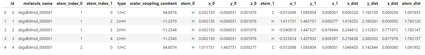
4.3. Label encoding
- type, atom_0, atom_1
# Label encoding
categorical_features = ['type', 'atom_0', 'atom_1']
for col in categorical_features:
    le = LabelEncoder()
    le.fit(list(train_dist[col].values) + list(test_dist[col].values))
    train_dist[col] = le.transform(list(train_dist[col].values))
    test_dist[col] = le.transform(list(test_dist[col].values))

train_le = train_dist.copy()
test_le = test_dist.copy()train_le.head()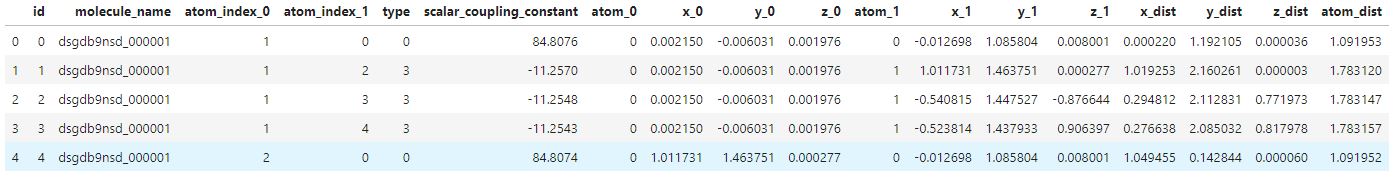
4.4. Standardization
- z = (x - u) / s
# train
train_data = train_le.drop(['id','molecule_name','scalar_coupling_constant'], axis=1)
train_target = train_le['scalar_coupling_constant']
# test
test_data = test_le.drop(['id','molecule_name',], axis=1)
# z-score standardization
train_scale = (train_data - train_data.mean()) / train_data.std()
train_scale = train_scale.fillna(0)
test_scale = (test_data - train_data.mean()) / train_data.std()4.5. Variable Correlations
train_corr = train_scale.copy()
train_corr['scalar_coupling_constant'] = train_target
corrmat = train_corr.corr()
top_corr_features = corrmat.index[abs(corrmat['scalar_coupling_constant']) >= 0.1]

plt.figure(figsize=(10,7))
sns.heatmap(train_corr[top_corr_features].corr(), annot=True, cmap="RdYlGn")
plt.title('Variable Correlations')
plt.show()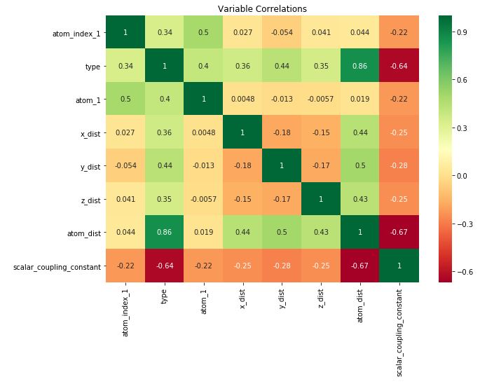
5. Training Model
5.1. Training by 'type' through LightGBM
train_scale = train_scale.drop('type', axis=1)
train_scale['type'] = train_tmp['type']
train_scale['scalar_coupling_constant'] = train_target

test_scale = test_scale.drop('type', axis=1)
test_scale[['id', 'type']] = test_tmp[['id', 'type']]
score_by_type = [] # List of Validation score by type
feature_importance_df = []
test_pred_df = pd.DataFrame(columns=['id', 'scalar_coupling_constant']) # Dataframe for submission
# Extract data by type
types = train_tmp['type'].unique()
for typ in types:
print('---Type of '+str(typ)+'---')
train = train_scale[train_scale['type'] == typ]
target = train['scalar_coupling_constant']
train = train.drop(['type','scalar_coupling_constant'], axis=1)
# Split train set / valid set
x_train, x_val, y_train, y_val = train_test_split(train, target, random_state=42)
# LightGBM
categorical_features = ['atom_0','atom_1']
lgb_train = lgb.Dataset(x_train, y_train, categorical_feature=categorical_features)
lgb_val = lgb.Dataset(x_val, y_val, categorical_feature=categorical_features)
# Parameters of LightGBM
params = {'num_leaves': 128,
'min_child_samples': 79,
'objective': 'regression',
'max_depth': 9,
'learning_rate': 0.1,
"boosting_type": "gbdt",
"subsample_freq": 1,
"subsample": 0.9,
"bagging_seed": 11,
"metric": 'mae',
"verbosity": -1,
'reg_alpha': 0.13,
'reg_lambda': 0.36,
'colsample_bytree': 1.0
}
# Training
lgb_model = lgb.train(params, lgb_train, valid_sets=[lgb_train, lgb_val],
num_boost_round=20000, # Number of boosting iterations.
early_stopping_rounds=500, # early stopping for valid set
verbose_eval=2500) # eval metric on the valid set is printed at 1000 each boosting
# Feature Importances
feature_importance = lgb_model.feature_importance()
df_fi = pd.DataFrame({'columns':x_train.columns, 'importances':feature_importance})
df_fi = df_fi[df_fi['importances'] > 0].sort_values(by=['importances'], ascending=False)
feature_importance_df.append(df_fi)
# Predict Validation set
score_by_type.append(list(lgb_model.best_score['valid_1'].values()))
# Predict Test set
test = test_scale[test_scale['type'] == typ]
test_id = test['id']
test = test.drop(['id','type'], axis=1)
test_preds = lgb_model.predict(test)
test_pred_df = pd.concat([test_pred_df, pd.DataFrame({'id':test_id, 'scalar_coupling_constant':test_preds})], axis=0)---Type of 1JHC---
Training until validation scores don't improve for 500 rounds.
[2500] training's l1: 2.77031 valid_1's l1: 3.67976
[5000] training's l1: 2.19648 valid_1's l1: 3.59536
[7500] training's l1: 1.81083 valid_1's l1: 3.56509
[10000] training's l1: 1.52513 valid_1's l1: 3.55207
[12500] training's l1: 1.30189 valid_1's l1: 3.54733
Early stopping, best iteration is:
[12398] training's l1: 1.31009 valid_1's l1: 3.54716
---Type of 2JHH---
Training until validation scores don't improve for 500 rounds.
[2500] training's l1: 0.599486 valid_1's l1: 0.930904
[5000] training's l1: 0.429952 valid_1's l1: 0.920848
Early stopping, best iteration is:
[6444] training's l1: 0.363731 valid_1's l1: 0.919744
---Type of 1JHN---
Training until validation scores don't improve for 500 rounds.
[2500] training's l1: 0.574269 valid_1's l1: 1.869
Early stopping, best iteration is:
[2790] training's l1: 0.51238 valid_1's l1: 1.86748
---Type of 2JHN---
Training until validation scores don't improve for 500 rounds.
[2500] training's l1: 0.493351 valid_1's l1: 1.29156
[5000] training's l1: 0.245368 valid_1's l1: 1.26562
[7500] training's l1: 0.136667 valid_1's l1: 1.25931
[10000] training's l1: 0.0806357 valid_1's l1: 1.25729
[12500] training's l1: 0.0501038 valid_1's l1: 1.25649
[15000] training's l1: 0.0325061 valid_1's l1: 1.25602
Early stopping, best iteration is:
[16603] training's l1: 0.025108 valid_1's l1: 1.25588
---Type of 2JHC---
Training until validation scores don't improve for 500 rounds.
[2500] training's l1: 1.45707 valid_1's l1: 1.78894
[5000] training's l1: 1.22333 valid_1's l1: 1.74951
[7500] training's l1: 1.0595 valid_1's l1: 1.734
[10000] training's l1: 0.931867 valid_1's l1: 1.72621
[12500] training's l1: 0.827693 valid_1's l1: 1.7222
[15000] training's l1: 0.740337 valid_1's l1: 1.72091
[17500] training's l1: 0.665914 valid_1's l1: 1.7203
Early stopping, best iteration is:
[17624] training's l1: 0.662523 valid_1's l1: 1.72024
---Type of 3JHH---
Training until validation scores don't improve for 500 rounds.
[2500] training's l1: 0.750457 valid_1's l1: 1.084
[5000] training's l1: 0.549578 valid_1's l1: 1.04283
[7500] training's l1: 0.427516 valid_1's l1: 1.02508
[10000] training's l1: 0.343351 valid_1's l1: 1.01595
[12500] training's l1: 0.281535 valid_1's l1: 1.01117
[15000] training's l1: 0.234395 valid_1's l1: 1.00805
[17500] training's l1: 0.197292 valid_1's l1: 1.00612
[20000] training's l1: 0.167506 valid_1's l1: 1.00516
Did not meet early stopping. Best iteration is:
[20000] training's l1: 0.167506 valid_1's l1: 1.00516
---Type of 3JHC---
Training until validation scores don't improve for 500 rounds.
[2500] training's l1: 1.14564 valid_1's l1: 1.35361
[5000] training's l1: 0.957949 valid_1's l1: 1.28948
[7500] training's l1: 0.830959 valid_1's l1: 1.2569
[10000] training's l1: 0.735763 valid_1's l1: 1.23707
[12500] training's l1: 0.65866 valid_1's l1: 1.22372
[15000] training's l1: 0.594712 valid_1's l1: 1.2142
[17500] training's l1: 0.540621 valid_1's l1: 1.2074
[20000] training's l1: 0.493743 valid_1's l1: 1.20232
Did not meet early stopping. Best iteration is:
[20000] training's l1: 0.493743 valid_1's l1: 1.20232
---Type of 3JHN---
Training until validation scores don't improve for 500 rounds.
[2500] training's l1: 0.231975 valid_1's l1: 0.513043
[5000] training's l1: 0.127354 valid_1's l1: 0.502675
[7500] training's l1: 0.0764305 valid_1's l1: 0.49964
[10000] training's l1: 0.0486108 valid_1's l1: 0.498466
[12500] training's l1: 0.0325766 valid_1's l1: 0.498049
[15000] training's l1: 0.0228697 valid_1's l1: 0.497765
[17500] training's l1: 0.0167369 valid_1's l1: 0.497581
[20000] training's l1: 0.0128106 valid_1's l1: 0.497526
Did not meet early stopping. Best iteration is:
[20000] training's l1: 0.0128106 valid_1's l1: 0.497526
5.2. Validation MAE by type
for typ, score in zip(types, score_by_type):
    print('Type {} valid MAE  : {}'.format(str(typ), score))

print('\nAverage of valid MAE  : {}'.format(np.mean(score_by_type)))
Type 1JHC valid MAE : [3.5471584407190475]
Type 2JHH valid MAE : [0.9197439377103146]
Type 1JHN valid MAE : [1.8674786631630775]
Type 2JHN valid MAE : [1.255876548899015]
Type 2JHC valid MAE : [1.7202390170123096]
Type 3JHH valid MAE : [1.0051635344922942]
Type 3JHC valid MAE : [1.2023186835296467]
Type 3JHN valid MAE : [0.4975260038664571]
Average of valid MAE : 1.5019381036740203
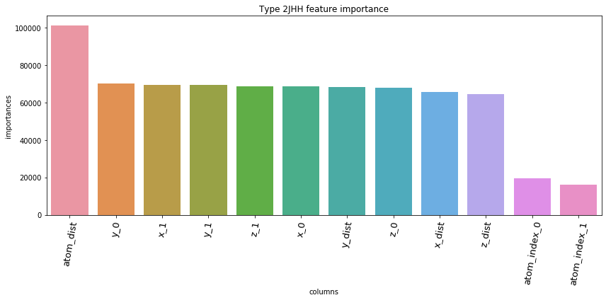
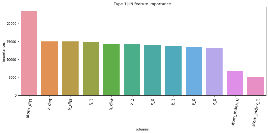
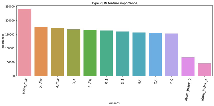
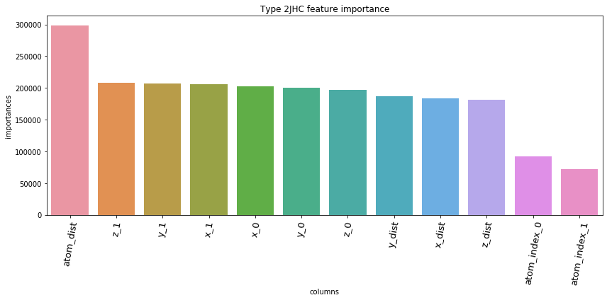
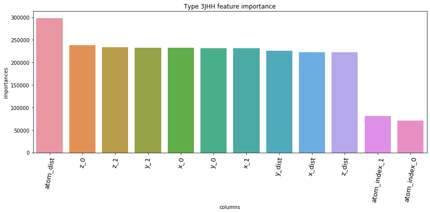
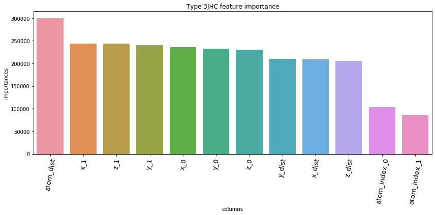
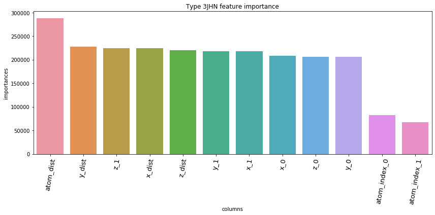
5.3. Feature Importances Plot by Type
for typ, df_fi in zip(types, feature_importance_df):
    fig = plt.figure(figsize=(12, 6))
    ax = sns.barplot(df_fi['columns'], df_fi['importances'])
    ax.set_xticklabels(df_fi['columns'], rotation=80, fontsize=13)
    plt.title('Type '+str(typ)+' feature importance')
    plt.tight_layout()
    plt.show()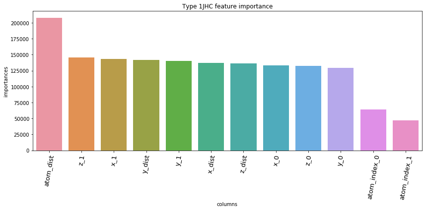
5.4. Save prediction of test set to *.csv
test_pred_df.head(10)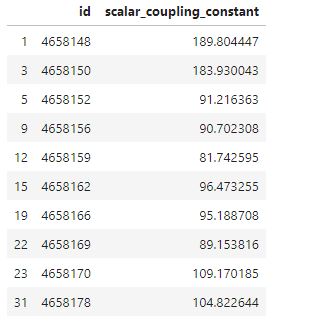
test_pred_df.to_csv('lgb_submission.csv', index=False)References
kaggle kernels
- https://www.kaggle.com/jesucristo/single-lgbm-2-242-top54
- https://www.kaggle.com/super13579/simple-eda-and-lightgbm
- https://www.kaggle.com/artgor/molecular-properties-eda-and-models
blog/docs
- https://gorakgarak.tistory.com/1285
- https://towardsdatascience.com/understanding-gradient-boosting-machines-using-xgboost-and-lightgbm-parameters-3af1f9db9700
- https://lightgbm.readthedocs.io/en/latest/
Outro
처음 예측 모델을 위해서 Neural Net을 이용하였었는데 default parameter의 Random Forest 알고리즘보다도 훨씬 낮은 성능을 보였다. 어느 글에서 말하길, 딥러닝이 항상 좋은 성능을 내지 않는다고 한다.
이런 Structured tabular 형태의 데이터에 neural net은 over-fitting 하는 경우가 많으며, 거의 대부분의 경우 xgboost나 lightgbm과 같은 gradient boosting 계열의 알고리즘이 잘 작동한다고 한다.(파라미터값을 잘 optimize 했을 때..)
앞으로 gbm 계열의 알고리즘에 대해 좀더 공부해봐야할 것 같다.
.jpeg)