
Intro
캐글의 고전적인 문제이며 머신러닝을 공부하는 사람이라면 누구나 한번쯤 다뤄봤을 Boston house price Dataset을 통해 regression하는 과정을 소개하려 한다. 정식 competition 명칭은 'House Prices: Advanced Regression Techniques'이며, 현재 누구나 submission을 제출할 수 있다.

위에서 말했듯이 boston house price데이터셋은 왠만한 머신러닝 공부하는 사람들은 한번쯤 봤을 것이며, 대부분의 머신러닝 입문 교재에도 꼭 한번씩은 소개가 되는 데이터셋이다. 하지만, 대부분의 교재나 강의에서는 이미 feature engineering을 거친 아주 잘 정형화 된(모델에 바로 적용 가능한)데이터셋을 사용하며 데이터 처리 과정은 생략하는 경우가 대부분인 것 같다. 하지만 boston house price 데이터셋은 무려 81개의 다양한 칼럼 변수를 가지고 있으며, 각 칼럼 특성에 맞는 전처리가 필요하다.
따라서, 여기서는 boston house price 데이터셋에 어떻게 적절한 feature engineering을 적용하고, 최근 kaggle에서 가장 인기 있는 모델인 XGBoost 모델을 어떻게 적용하였는지 소개한다.
Import Library
import numpy as np
import pandas as pd
import matplotlib.pyplot as plt
import seaborn as sns
1. Load Data
- 데이터의 경우 train, test set이 분리되어 제공되며 test set에 대한 예측결과가 추후 submission으로 제출된다.
- train 데이터의 경우 1,460건, test 데이터가 1459건이며 총 81개의 칼럼을 가진다.
# laod data
train_df = pd.read_csv('house_train.csv')
test_df = pd.read_csv('house_test.csv')

train_df.head()| Id | MSSubClass | MSZoning | LotFrontage | LotArea | Street | Alley | LotShape | LandContour | Utilities | ... | PoolArea | PoolQC | Fence | MiscFeature | MiscVal | MoSold | YrSold | SaleType | SaleCondition | SalePrice | |
|---|---|---|---|---|---|---|---|---|---|---|---|---|---|---|---|---|---|---|---|---|---|
| 0 | 1 | 60 | RL | 65.0 | 8450 | Pave | NaN | Reg | Lvl | AllPub | ... | 0 | NaN | NaN | NaN | 0 | 2 | 2008 | WD | Normal | 208500 |
| 1 | 2 | 20 | RL | 80.0 | 9600 | Pave | NaN | Reg | Lvl | AllPub | ... | 0 | NaN | NaN | NaN | 0 | 5 | 2007 | WD | Normal | 181500 |
| 2 | 3 | 60 | RL | 68.0 | 11250 | Pave | NaN | IR1 | Lvl | AllPub | ... | 0 | NaN | NaN | NaN | 0 | 9 | 2008 | WD | Normal | 223500 |
| 3 | 4 | 70 | RL | 60.0 | 9550 | Pave | NaN | IR1 | Lvl | AllPub | ... | 0 | NaN | NaN | NaN | 0 | 2 | 2006 | WD | Abnorml | 140000 |
| 4 | 5 | 60 | RL | 84.0 | 14260 | Pave | NaN | IR1 | Lvl | AllPub | ... | 0 | NaN | NaN | NaN | 0 | 12 | 2008 | WD | Normal | 250000 |
5 rows × 81 columns
# set index
train_df.set_index('Id', inplace=True)
test_df.set_index('Id', inplace=True)
len_train_df = len(train_df)
len_test_df = len(test_df)
2. Feature Selection - Variables of Corrleation >= 0.3
- 고려해야 할 변수가 많을 땐 각 독립변수와 종속변수 간의 상관관계(Corrleation)을 검토해보는 것이 좋다.
- 모든 변수를 사용하는 것도 좋지만 그 중 좀더 의미 있는 변수만을 골라내어 모델을 구축하는 것이 모델의 예측 정확도를 높이는 방법이다.
- corr()함수를 통해 dataframe내의 모든 변수간의 상관관계를 그린 후 상관관계가 0.3이상인 변수만 heatmap으로 출력하였다.
corrmat = train_df.corr()
top_corr_features = corrmat.index[abs(corrmat["SalePrice"])>=0.3]
top_corr_features
Index(['LotFrontage', 'OverallQual', 'YearBuilt', 'YearRemodAdd', 'MasVnrArea',
'BsmtFinSF1', 'TotalBsmtSF', '1stFlrSF', '2ndFlrSF', 'GrLivArea',
'FullBath', 'TotRmsAbvGrd', 'Fireplaces', 'GarageYrBlt', 'GarageCars',
'GarageArea', 'WoodDeckSF', 'OpenPorchSF', 'SalePrice'],
dtype='object')# heatmap
plt.figure(figsize=(13,10))
g = sns.heatmap(train_df[top_corr_features].corr(),annot=True,cmap="RdYlGn")
# feature selection
# train_df = train_df[top_corr_features]
# test_df = test_df[top_corr_features.drop(['SalePrice'])]
# split y_label
train_y_label = train_df['SalePrice'] # target 값을 미리 분리하였음.
train_df.drop(['SalePrice'], axis=1, inplace=True)3. Concat train & test set
- train과 test 셋에 동일한 feature engineering을 적용해주기 위해 우선 두개의 데이터 셋을 하나로 합쳐주었다.
- 합쳐주니 2,919개로 데이터가 늘었다.
# concat train & test
boston_df = pd.concat((train_df, test_df), axis=0)
boston_df_index = boston_df.index

print('Length of Boston Dataset : ',len(boston_df))
boston_df.head()
Length of Boston Dataset : 2919| MSSubClass | MSZoning | LotFrontage | LotArea | Street | Alley | LotShape | LandContour | Utilities | LotConfig | ... | ScreenPorch | PoolArea | PoolQC | Fence | MiscFeature | MiscVal | MoSold | YrSold | SaleType | SaleCondition | |
|---|---|---|---|---|---|---|---|---|---|---|---|---|---|---|---|---|---|---|---|---|---|
| Id | |||||||||||||||||||||
| 1 | 60 | RL | 65.0 | 8450 | Pave | NaN | Reg | Lvl | AllPub | Inside | ... | 0 | 0 | NaN | NaN | NaN | 0 | 2 | 2008 | WD | Normal |
| 2 | 20 | RL | 80.0 | 9600 | Pave | NaN | Reg | Lvl | AllPub | FR2 | ... | 0 | 0 | NaN | NaN | NaN | 0 | 5 | 2007 | WD | Normal |
| 3 | 60 | RL | 68.0 | 11250 | Pave | NaN | IR1 | Lvl | AllPub | Inside | ... | 0 | 0 | NaN | NaN | NaN | 0 | 9 | 2008 | WD | Normal |
| 4 | 70 | RL | 60.0 | 9550 | Pave | NaN | IR1 | Lvl | AllPub | Corner | ... | 0 | 0 | NaN | NaN | NaN | 0 | 2 | 2006 | WD | Abnorml |
| 5 | 60 | RL | 84.0 | 14260 | Pave | NaN | IR1 | Lvl | AllPub | FR2 | ... | 0 | 0 | NaN | NaN | NaN | 0 | 12 | 2008 | WD | Normal |
5 rows × 79 columns
4. Check NaN ratio and Remove null ratio >= 0.5
- 데이터를 처리할 때 항상 Null값을 어떻게 처리할지 고민해야 한다. 추후 모델에 입력되는 input값에는 절대 어떠한 Null 값이 있어서는 안되며 있더라도 에러가 발생하기 때문에 미리 꼭 처리해주어야 한다.
- 우선 각 칼럼별로 Null값 비율이 50%이상인 칼럼을 찾아 해당 칼럼을 제거해주었다.
- 보통 null값 처리를 위해 평균, 최대값, 최소값 등으로 대체하곤 하는데 위와 같이 대부분의 칼럼이 Null인 데이터는 차라리 없애주는 것이 좋다.
# check null
check_null = boston_df.isna().sum() / len(boston_df)

# columns of null ratio >= 0.5
check_null[check_null >= 0.5]
Alley 0.932169
PoolQC 0.996574
Fence 0.804385
MiscFeature 0.964029
dtype: float64# remove columns of null ratio >= 0.5
remove_cols = check_null[check_null >= 0.5].keys()
boston_df = boston_df.drop(remove_cols, axis=1)
boston_df.head()| MSSubClass | MSZoning | LotFrontage | LotArea | Street | LotShape | LandContour | Utilities | LotConfig | LandSlope | ... | OpenPorchSF | EnclosedPorch | 3SsnPorch | ScreenPorch | PoolArea | MiscVal | MoSold | YrSold | SaleType | SaleCondition | |
|---|---|---|---|---|---|---|---|---|---|---|---|---|---|---|---|---|---|---|---|---|---|
| Id | |||||||||||||||||||||
| 1 | 60 | RL | 65.0 | 8450 | Pave | Reg | Lvl | AllPub | Inside | Gtl | ... | 61 | 0 | 0 | 0 | 0 | 0 | 2 | 2008 | WD | Normal |
| 2 | 20 | RL | 80.0 | 9600 | Pave | Reg | Lvl | AllPub | FR2 | Gtl | ... | 0 | 0 | 0 | 0 | 0 | 0 | 5 | 2007 | WD | Normal |
| 3 | 60 | RL | 68.0 | 11250 | Pave | IR1 | Lvl | AllPub | Inside | Gtl | ... | 42 | 0 | 0 | 0 | 0 | 0 | 9 | 2008 | WD | Normal |
| 4 | 70 | RL | 60.0 | 9550 | Pave | IR1 | Lvl | AllPub | Corner | Gtl | ... | 35 | 272 | 0 | 0 | 0 | 0 | 2 | 2006 | WD | Abnorml |
| 5 | 60 | RL | 84.0 | 14260 | Pave | IR1 | Lvl | AllPub | FR2 | Gtl | ... | 84 | 0 | 0 | 0 | 0 | 0 | 12 | 2008 | WD | Normal |
5 rows × 75 columns
5. Check Object & Numeric variables
- 해당 데이터 셋에는 수치형 데이터만 있는 것이 아니다. [성별: 남자, 여자], [학급: 햇님반, 꽃님반, 달님반]과 같은 카테고리형 데이터도 존재한다.
- 이러한 카테고리형 데이터는 각 칼럼을 0과 1로 변환해주는 one-hot encoding을 적용해주어 수치값과 가중치를 달리해주어야 한다.
- 수치형 데이터와 카테고리형 데이터를 구분하기 위해 select_dtypes()를 이용하였다. parameter값으로 include와 exclude를 적용할 수 있는데 이를 통해 데이터를 분리한다.
# split object & numeric
boston_obj_df = boston_df.select_dtypes(include='object')	# 카테고리형
boston_num_df = boston_df.select_dtypes(exclude='object') # 수치형print('Object type columns:\n',boston_obj_df.columns)
print('---------------------------------------------------------------------------------')
print('Numeric type columns:\n',boston_num_df.columns)Object type columns:
Index(['MSZoning', 'Street', 'LotShape', 'LandContour', 'Utilities',
'LotConfig', 'LandSlope', 'Neighborhood', 'Condition1', 'Condition2',
'BldgType', 'HouseStyle', 'RoofStyle', 'RoofMatl', 'Exterior1st',
'Exterior2nd', 'MasVnrType', 'ExterQual', 'ExterCond', 'Foundation',
'BsmtQual', 'BsmtCond', 'BsmtExposure', 'BsmtFinType1', 'BsmtFinType2',
'Heating', 'HeatingQC', 'CentralAir', 'Electrical', 'KitchenQual',
'Functional', 'FireplaceQu', 'GarageType', 'GarageFinish', 'GarageQual',
'GarageCond', 'PavedDrive', 'SaleType', 'SaleCondition'],
dtype='object')
---------------------------------------------------------------------------------
Numeric type columns:
Index(['MSSubClass', 'LotFrontage', 'LotArea', 'OverallQual', 'OverallCond',
'YearBuilt', 'YearRemodAdd', 'MasVnrArea', 'BsmtFinSF1', 'BsmtFinSF2',
'BsmtUnfSF', 'TotalBsmtSF', '1stFlrSF', '2ndFlrSF', 'LowQualFinSF',
'GrLivArea', 'BsmtFullBath', 'BsmtHalfBath', 'FullBath', 'HalfBath',
'BedroomAbvGr', 'KitchenAbvGr', 'TotRmsAbvGrd', 'Fireplaces',
'GarageYrBlt', 'GarageCars', 'GarageArea', 'WoodDeckSF', 'OpenPorchSF',
'EnclosedPorch', '3SsnPorch', 'ScreenPorch', 'PoolArea', 'MiscVal',
'MoSold', 'YrSold'],
dtype='object')6. Change object type to dummy variables
- 위에서 분리한 카테고리형 데이터에 one-hot encoding을 적용하기 위해 pandas의 pd.get_dummies()를 적용하였다. one-hot encoding 적용시 [남자, 여자]의 경우 [[1,0], [0,1]]과 같은 형태로 변환된다.
boston_dummy_df = pd.get_dummies(boston_obj_df, drop_first=True)
boston_dummy_df.index = boston_df_index
boston_dummy_df.head()| MSZoning_FV | MSZoning_RH | MSZoning_RL | MSZoning_RM | Street_Pave | LotShape_IR2 | LotShape_IR3 | LotShape_Reg | LandContour_HLS | LandContour_Low | ... | SaleType_ConLI | SaleType_ConLw | SaleType_New | SaleType_Oth | SaleType_WD | SaleCondition_AdjLand | SaleCondition_Alloca | SaleCondition_Family | SaleCondition_Normal | SaleCondition_Partial | |
|---|---|---|---|---|---|---|---|---|---|---|---|---|---|---|---|---|---|---|---|---|---|
| Id | |||||||||||||||||||||
| 1 | 0 | 0 | 1 | 0 | 1 | 0 | 0 | 1 | 0 | 0 | ... | 0 | 0 | 0 | 0 | 1 | 0 | 0 | 0 | 1 | 0 |
| 2 | 0 | 0 | 1 | 0 | 1 | 0 | 0 | 1 | 0 | 0 | ... | 0 | 0 | 0 | 0 | 1 | 0 | 0 | 0 | 1 | 0 |
| 3 | 0 | 0 | 1 | 0 | 1 | 0 | 0 | 0 | 0 | 0 | ... | 0 | 0 | 0 | 0 | 1 | 0 | 0 | 0 | 1 | 0 |
| 4 | 0 | 0 | 1 | 0 | 1 | 0 | 0 | 0 | 0 | 0 | ... | 0 | 0 | 0 | 0 | 1 | 0 | 0 | 0 | 0 | 0 |
| 5 | 0 | 0 | 1 | 0 | 1 | 0 | 0 | 0 | 0 | 0 | ... | 0 | 0 | 0 | 0 | 1 | 0 | 0 | 0 | 1 | 0 |
5 rows × 200 columns
7. Impute NaN of numeric data to 'mean'
- 4번쨰 과정에서 null값이 50%이상인 변수들을 제거해주었었는데, 그 이하로 null값이 있는 데이터를 마저 처리해주어야 한다.
- 여기서는 각 칼럼의 null값을 해당하는 각 변수들의 평균(mean)으로 대체(imputation)해주었다.
- 평균값 대체를 위하여 scikit-learn의 Imputer 함수를 이용하였으며, strategy 값에 대체해주고자 하는 이름을 넣어주면 해당 값으로 처리한다.
from sklearn.preprocessing import Imputer

imputer = Imputer(strategy='mean')
imputer.fit(boston_num_df)
boston_num_df_ = imputer.transform(boston_num_df)
boston_num_df = pd.DataFrame(boston_num_df_, columns=boston_num_df.columns, index=boston_df_index)
boston_num_df.head()| MSSubClass | LotFrontage | LotArea | OverallQual | OverallCond | YearBuilt | YearRemodAdd | MasVnrArea | BsmtFinSF1 | BsmtFinSF2 | ... | GarageArea | WoodDeckSF | OpenPorchSF | EnclosedPorch | 3SsnPorch | ScreenPorch | PoolArea | MiscVal | MoSold | YrSold | |
|---|---|---|---|---|---|---|---|---|---|---|---|---|---|---|---|---|---|---|---|---|---|
| Id | |||||||||||||||||||||
| 1 | 60.0 | 65.0 | 8450.0 | 7.0 | 5.0 | 2003.0 | 2003.0 | 196.0 | 706.0 | 0.0 | ... | 548.0 | 0.0 | 61.0 | 0.0 | 0.0 | 0.0 | 0.0 | 0.0 | 2.0 | 2008.0 |
| 2 | 20.0 | 80.0 | 9600.0 | 6.0 | 8.0 | 1976.0 | 1976.0 | 0.0 | 978.0 | 0.0 | ... | 460.0 | 298.0 | 0.0 | 0.0 | 0.0 | 0.0 | 0.0 | 0.0 | 5.0 | 2007.0 |
| 3 | 60.0 | 68.0 | 11250.0 | 7.0 | 5.0 | 2001.0 | 2002.0 | 162.0 | 486.0 | 0.0 | ... | 608.0 | 0.0 | 42.0 | 0.0 | 0.0 | 0.0 | 0.0 | 0.0 | 9.0 | 2008.0 |
| 4 | 70.0 | 60.0 | 9550.0 | 7.0 | 5.0 | 1915.0 | 1970.0 | 0.0 | 216.0 | 0.0 | ... | 642.0 | 0.0 | 35.0 | 272.0 | 0.0 | 0.0 | 0.0 | 0.0 | 2.0 | 2006.0 |
| 5 | 60.0 | 84.0 | 14260.0 | 8.0 | 5.0 | 2000.0 | 2000.0 | 350.0 | 655.0 | 0.0 | ... | 836.0 | 192.0 | 84.0 | 0.0 | 0.0 | 0.0 | 0.0 | 0.0 | 12.0 | 2008.0 |
5 rows × 36 columns
8. Merge numeric_df & dummies_df
- 위에서 각각 처리한 카테고리형 데이터와 수치형 데이터를 이제 최종적으로 다시 하나로 merge해준다. merge시 index 순서가 꼬이지 않게 left_index=True, right_index=True를 지정하여 merge를 수행한다.
boston_df = pd.merge(boston_dummy_df, boston_num_df, left_index=True, right_index=True)
boston_df.head()| MSZoning_FV | MSZoning_RH | MSZoning_RL | MSZoning_RM | Street_Pave | LotShape_IR2 | LotShape_IR3 | LotShape_Reg | LandContour_HLS | LandContour_Low | ... | GarageArea | WoodDeckSF | OpenPorchSF | EnclosedPorch | 3SsnPorch | ScreenPorch | PoolArea | MiscVal | MoSold | YrSold | |
|---|---|---|---|---|---|---|---|---|---|---|---|---|---|---|---|---|---|---|---|---|---|
| Id | |||||||||||||||||||||
| 1 | 0 | 0 | 1 | 0 | 1 | 0 | 0 | 1 | 0 | 0 | ... | 548.0 | 0.0 | 61.0 | 0.0 | 0.0 | 0.0 | 0.0 | 0.0 | 2.0 | 2008.0 |
| 2 | 0 | 0 | 1 | 0 | 1 | 0 | 0 | 1 | 0 | 0 | ... | 460.0 | 298.0 | 0.0 | 0.0 | 0.0 | 0.0 | 0.0 | 0.0 | 5.0 | 2007.0 |
| 3 | 0 | 0 | 1 | 0 | 1 | 0 | 0 | 0 | 0 | 0 | ... | 608.0 | 0.0 | 42.0 | 0.0 | 0.0 | 0.0 | 0.0 | 0.0 | 9.0 | 2008.0 |
| 4 | 0 | 0 | 1 | 0 | 1 | 0 | 0 | 0 | 0 | 0 | ... | 642.0 | 0.0 | 35.0 | 272.0 | 0.0 | 0.0 | 0.0 | 0.0 | 2.0 | 2006.0 |
| 5 | 0 | 0 | 1 | 0 | 1 | 0 | 0 | 0 | 0 | 0 | ... | 836.0 | 192.0 | 84.0 | 0.0 | 0.0 | 0.0 | 0.0 | 0.0 | 12.0 | 2008.0 |
5 rows × 236 columns
9. Split train & validation & test set
- 모델 학습 및 검증을 위해 데이터를 split한다.
- 여기서 test set의 경우 정답값이 없는 예측해야 하는 값이므로 검증을 위해 validation set을 train set의 20%만큼을 지정해주었다.
- 최종적으로 1,168개의 데이터로 학습 및 292개의 데이터로 검증 후 1,459개의 test셋을 예측한다.
train_df = boston_df[:len_train_df]
test_df = boston_df[len_train_df:]

train_df['SalePrice'] = train_y_label

print('train set length: ',len(train_df))
print('test set length: ',len(test_df))
train set length: 1460
test set length: 1459from sklearn.model_selection import train_test_split
X_train = train_df.drop(['SalePrice'], axis=1)
y_train = train_df['SalePrice']
X_train, X_val, y_train, y_val = train_test_split(X_train, y_train, test_size=0.2, shuffle=True)
X_test = test_df
test_id_idx = test_df.indexprint('X_train : ',len(X_train))
print('X_val : ',len(X_val))
print('X_test :',len(X_test))X_train : 1168
X_val : 292
X_test : 145910. Training by XGBRegression Model
- 모델 학습을 위해 최근 kaggle에서 가장 인기 있는 모델인 XGBoost 모델을 이용하였다. 해당 예측은 regression 예측이므로 XGBRegressor() 모델을 이용하였다.
- 최적의 모델 파라미터 설정을 위하여 GridSearch를 이용하였으며, 5번의 cross-validation으로 검증을 진행하였다.
- 학습 후 bestparams를 출력하면 최적의 파라미터 값이 출력된다.
from sklearn.model_selection import GridSearchCV
import xgboost as xgb

param = {
    'max_depth':[2,3,4],
    'n_estimators':range(550,700,50),
    'colsample_bytree':[0.5,0.7,1],
    'colsample_bylevel':[0.5,0.7,1],
}
model = xgb.XGBRegressor()
grid_search = GridSearchCV(estimator=model, param_grid=param, cv=5,
                           scoring='neg_mean_squared_error',
                           n_jobs=-1)

grid_search.fit(X_train, y_train)
print(grid_search.best_params_)
print(grid_search.best_estimator_)
{'colsample_bylevel': 0.5, 'colsample_bytree': 0.7, 'max_depth': 3, 'n_estimators': 600}
XGBRegressor(base_score=0.5, booster='gbtree', colsample_bylevel=0.5,
colsample_bytree=0.7, gamma=0, learning_rate=0.1, max_delta_step=0,
max_depth=3, min_child_weight=1, missing=None, n_estimators=600,
n_jobs=1, nthread=None, objective='reg:linear', random_state=0,
reg_alpha=0, reg_lambda=1, scale_pos_weight=1, seed=None,
silent=True, subsample=1)11. Prediction & Score
- 검증을 위해 Mean Absolute Error(MAE) 지표를 활용하였다. MSE를 활용할 경우 error값이 클 경우 그에 제곱된 값이 출력되기 때문에 값이 너무 커져 보기 불편하다는 단점이 있다.
- 검증 결과 validation mae 값이 14,000정도인데, 워낙 집 가격에 대한 값의 범위가 넓기 때문에 이 정도 error값은 심각한 정도는 아니며 납득할만한 수준이라고 할 수 있다.
from sklearn.metrics import mean_squared_error, mean_absolute_error
pred_train = grid_search.predict(X_train)
pred_val = grid_search.predict(X_val)

print('train mae score: ', mean_absolute_error(y_train, pred_train))
print('val mae score:', mean_absolute_error(y_val, pred_val))
train mae score: 4790.379391186858
val mae score: 14178.155835295376- 이후 validation set을 대상으로 예측을 수행한 후 실제 값과의 결과를 plotting하였다. - 어느 정도 경향을 잘 예측하고 있는 것을 확인할 수 있다.
plt.figure(figsize=(17,7))
plt.plot(range(0, len(y_val)), y_val,'o-', label='Validation Actual')
plt.plot(range(0, len(pred_val)), pred_val, '-', label='Validation Predict')
plt.title('Prediction of House Prices')
plt.ylabel('Prices')
plt.legend()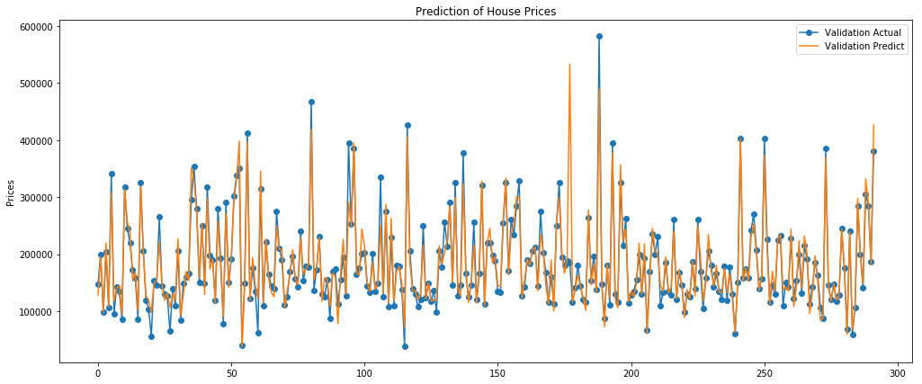
12. Predict test set & Submit submission.csv
test_y_pred = grid_search.predict(X_test)id_pred_df = pd.DataFrame()
id_pred_df['Id'] = test_id_idx
id_pred_df['SalePrice'] = test_y_predid_pred_df.to_csv('submission.csv', index=False)Outro
실제 submission에서 성능 평가 시에는 Root Mean Squarred Error이용하는데, 제출 결과 0.12875로 총 4,465팀 중 1,867등을 기록하였다(상위 42%). 이번에는 단순히 테스트를 위해 머신러닝 모델만 적용해보았는데, LSTM 모델을 적용하면 확실히 더 낮은 error 값이 나올 것으로 기대된다.
.jpeg)