[ML] California Housing Prices

🌐 Overview

The objective of working with the California Housing Prices dataset is to predict median housing prices of California districts based on a set of features. This is a regression problem where the goal is to model the relationship between housing prices (the target variables) and various features(predictors).

📊 Usage Dataset

Column Name	Description	Type	Example Value
MedInc	Median income of households (scaled)	Continuous	3.87
HouseAge	Median age of houses in the block group	Continuous	15
AveRooms	Average number of rooms per household	Continuous	6.98
AveBedrms	Average number of bedrooms per household	Continuous	1.02
Population	Total population in the block group	Continuous	322
AveOccup	Average number of people per household	Continuous	2.56
Latitude	Geographical latitude of the block group	Continuous	37.88
Longitude	Geographical longitude of the block group	Continuous	-122.23
MedHouseVal	Median house value (in $100,000s) (Target)	Continuous	4.52

• Target variables : MedHouseVal (Median house value for households in the block group)
• Includes approximately 20,640 observations.
• Features are numeric and mostly continuous.
• Target variable is also continuous.

🔍 Simple Linear Regression EDA

1. Data load

import pandas as pd
import numpy as np
import matplotlib.pyplot as plt
from sklearn.datasets import fetch_california_housing
from sklearn.model_selection import train_test_split
from sklearn.linear_model import LinearRegression
from sklearn.metrics import mean_squared_error, r2_score

california = fetch_california_housing()
X = pd.DataFrame(california.data, columns=california.feature_names)
y = california.target  

• X : Independent variables(features)
• y : Dependent variable(target) in 1D array

print(X.head())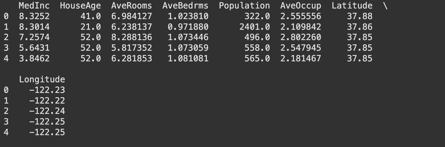

print(y[:5])
# Prints the first 5 values of the target variable y.
# [4.526 3.585 3.521 3.413 3.422]

X_simple = X[['MedInc']]

2. Split the dataset

X_train, X_test, y_train, y_test = train_test_split(X_simple, y, test_size=0.2, random_state=42)

• random_state = 42 means that the same split will occur each time the code is run, making experiments consistent. The number doesn't matter. You can put any numbers.

• output

  • X_train: The training data (80% of X_simple).
  • X_test: The testing data (20% of X_simple).
  • y_train: The training labels (80% of y).
  • y_test: The testing labels (20% of y).

3. Training a model

model = LinearRegression()
model.fit(X_train, y_train)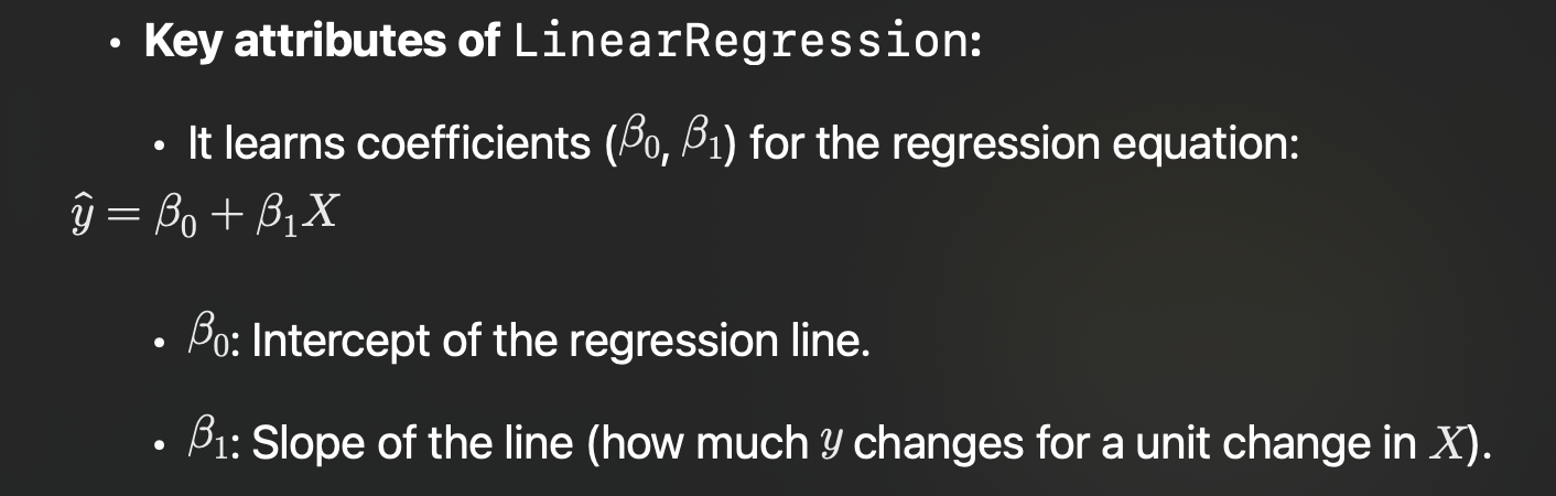

• model.fit(X_train, y_train) means that it fits the linear regression model to the training data. The fit method
  • X_train : Training data for the independent variable(s). In this case, it's the single column MedInc from the training set.
  • y_train : Training data for the dependent variable(y), which is the median house value.
  • This step trains the linear regression model to find the relationship between MedInc and mdedian house value

4. Make predictions

y_pred = model.predict(X_test)

• Use the trained model to predict values for the test set
• Compare the predicted values(y_pred) against the true values (y_test) using metrics like, MAE, MSE, R-squared
• For example, if intercept is 1.5 and coefficient is 0.8, the euqation for predicting house prices became y = 1.5 + 0.8MedInc. This means for every unit increase in MedInc, the hosuse value increases by 0.8

5. Evaluate the performance

mse = mean_squared_error(y_test, y_pred)
r2 = r2_score(y_test, y_pred)

print(f"\nMean Squared Error: {mse:.2f}")
print(f"R-squared: {r2:.2f}")
# Mean Squared Error: 0.71
# R-squared: 0.46

• ⭐ ⭐ MSE(0.71) the squared prediction error. The root mean suqared error(RMSE) would be 0.84. So, the model’s predictions deviate from the actual house prices by approximately $84,000, on average. It is relatively high, suggesting room for improvement.
• R-squared(0.46) is insufficient to fully model the relationship.

6. Visulization

plt.scatter(X_test, y_test, color='blue', label='Actual Data')
plt.plot(X_test, y_pred, color='red', label='Regression Line')
plt.title("Linear Regression: MedInc vs House Value")
plt.xlabel("Median Income")
plt.ylabel("Median House Value")
plt.legend()
plt.show()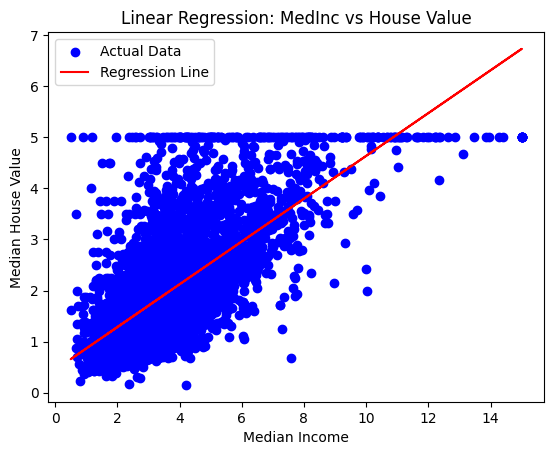

• The scatter and saturation at higher house values indicate that a simple linear regression may not fully capture the complexity of the relationship.
• There may be other factors (e.g., location, population) influencing house prices that are not included in this model.
• Let's condider trying a nonlinear regression model or polynomial regresion
• Include additional features (e.g., location, house age) to improve predictions.

🔍 Multiple Linear Regression EDA

1. Data load

california = fetch_california_housing()
X = pd.DataFrame(california.data, columns=california.feature_names)
y = california.target 

# select variables
X_selected = X[['MedInc', 'HouseAge', 'AveRooms', 'AveOccup']]

2. Split the dataset

X_train, X_test, y_train, y_test = train_test_split(X_selected, y, test_size=0.2, random_state=42)

3. Training a model

model = LinearRegression()
model.fit(X_train, y_train)

4. Make predictions

y_pred = model.predict(X_test)

5. Evaluate the performance

mse = mean_squared_error(y_test, y_pred)
r2 = r2_score(y_test, y_pred)

print(f"Mean Squared Error: {mse:.2f}")
print(f"R-squared: {r2:.2f}")
# Mean Squared Error: 0.66
# R-squared: 0.50

6. Visulization

plt.scatter(y_test, y_pred, color='blue', alpha=0.6)
plt.plot([0, 5], [0, 5], color='red', linestyle='--')  # 1:1 선
plt.title("Actual vs Predicted Values")
plt.xlabel("Actual Median House Value")
plt.ylabel("Predicted Median House Value")
plt.show()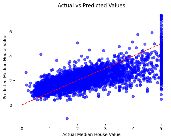

• By incorporating additional features, the model accounts for more variability in house prices, as shown by the closer clustering of points around the diagonal line.
• While it performs better, multiple regression models are harder to interpret due to the involvement of several features.
• Some points are far from the red dashed line, indicating that the model still has errors or might struggle with certain data points

🧩 Problem Definition

The goal is to predict the median housing value(MedHouseVal) of California district based on demographic and geographic attributes. This is a supervised regression problem, as the target variable is continuous.

🔍 Problem Identification

• Housing prices show nonlinear patterns (e.g., saturation at higher values) that simple linear regression may not capture.
• There are multiple factors beyond income that influence house prices, such as house age, average rooms, and population density.
• The dataset has an upper bound on house prices (capping at a value of 5), introducing potential bias.

💡 Hypothesis and Experimental Design

Simple Linear Regression

• Hypothesis: Median income (MedInc) is a strong predictor of median house value, and a simple linear model will provide reasonable predictions.
• Null Hypothesis: There is no linear relationship between MedInc and Median House Value.

Multiple Linear Regression

• Hypothesis: Incorporating additional features (e.g., house age, number of rooms, population) will significantly improve the model’s ability to explain variability in housing prices.
• Null Hypothesis: Adding more features does not improve model performance significantly.

✅ Validation

Simple Linear Regression:

• A clear positive correlation between MedInc and Median House Value.
• The model captures the general trend but leaves significant residual errors due to factors it cannot explain.
• R^2 : Likely low to moderate, indicating that MedInc alone explains some, but not most, of the variation in house prices.
• Validation Metric: Moderate R^2 value and relatively high MSE suggest limited accuracy.

Multiple Linear Regression:

• Adding more features significantly improves R^2 and reduces MSE.
• The model better captures the complexity of house price variability but may still struggle with saturation effects and potential outliers.
• R^2 : Higher than the simple regression model, indicating better explanatory power.
• Validation Metric: Lower MSE and higher R^2 validate the improved performance of the multiple regression model.

🔄 Retrospective

• If the goal is interpretability and simplicity, Simple Linear Regression is better. It shows a straightforward relationship between MedInc and house prices.
• If the goal is better prediction and accuracy, Multiple Linear Regression is better. It leverages more features, providing a closer match between predicted and actual values.

https://www.kaggle.com/datasets/camnugent/california-housing-prices