'Collaborative Score Distillation for Consistent Visual Synthesis' Paper Summary

Abstract

  Stein Variational Gradient Descent (SVGD)를 기반으로 한 Collaborative Score Distillation (CSD) 모델 제안. 여러 샘플을 SVGD의 'particle'로 여겨 score function을 합산하는 방법으로 inter-sample consistency를 향상시킴.

---

1. Introduction

  "Adapting the knowledge of pre-trained text-to-image diffusion models to more complex high-dimensional visual generative tasks beyond 2D images without modifying diffusion models using modality-specific training data."

• Modality-Specific Consistency

  • High-Resolution Images $\rarr$ Spatial Consistency
  • Video $\rarr$ Temporal consistency
  • 3D scene $\rarr$ View consistency
    : No built-in capability to ensure consistency in image diffusion models.

• Score Distillation Sampling (SDS)
  : Generative sampling을 pre-trained diffusion density scores에 대한 distillation으로 임의의 미분 가능한 operator에 대한 최적화를 가능케 해줌.

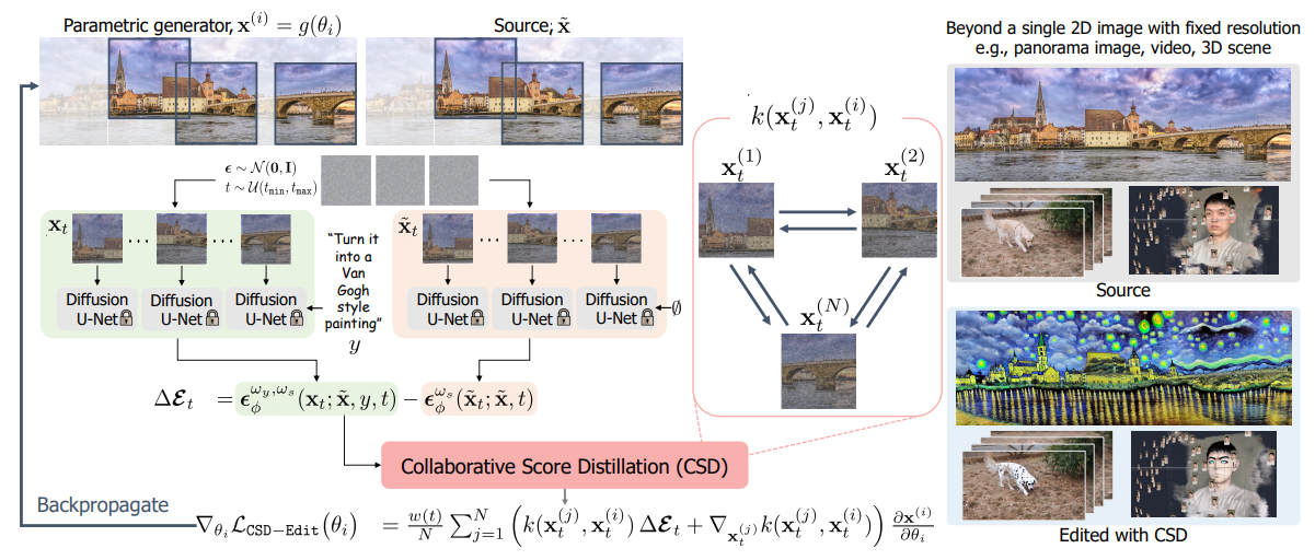
Collaborative Score Distillation (CSD)

• Generalization of SDS using SVGD $\rarr$ Inter-Sample Consistency
• CSD-Edit $\rarr$ CSD + Instruct-Pix2Pix

---

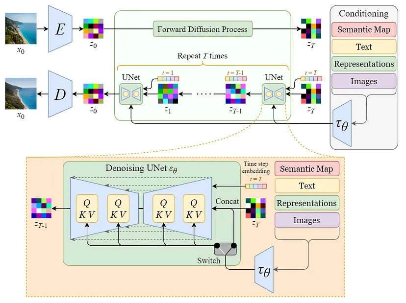
2. Preliminaries

• Diffusion Models
  : Basic diffusion models + Classifier-Free Guidance (CFG) + Instruct-Pix2Pix

• Score Distillation Sampling (SDS)
  : Density distillation loss

  $L_{\text{Distill}}(\theta; x=g(\theta))=E_{t,\epsilon}[\alpha_t/\sigma_tD_{\text{KL}}(q(x_t|x=g(\theta))||p_\phi^\omega(x_t;y,t))]$
  $\nabla_\theta L_{\text{SDS}}(\theta;x=g(\theta))=E_{t,\epsilon}[w(t)(\epsilon_\phi^\omega(x_t;y,t)-\epsilon)\frac{\partial x}{\partial \theta}]$

  : Dreamfusion 논문에서 제시. Dream Fields가 prompt와 rendered view 간 CLIP image-text similarity prior를 leverage한데 비해, Dreamfusion에서는 Imagen 등의 text-to-image diffusion model의 (spatial 정보가 보존된) gradient로 differentiable generator(NeRF)를 학습.
  : 이때, U-Net Jacobian term을 제외하여 연산량 및 모델 성능 개선.

• Stein Variational Gradient Descent (SVGD)
  : 기존의 variational inference 방법론은 주어진 입출력 데이터에 대한 posterior $p(w|D)$를 파라미터 $\theta$로 구성된 $q(w|\theta)$로 직접 근사. SVGD는 $w$와 동일한 차원의 feature를 갖는 particle이 posterior와 비슷한 분포를 갖도록 이동시켜 그로부터 얻어지는 empirical distribution을 활용.
  : Stein Discrepancy - Stein operator로 smooth vector function $f$를 함수 $p$에 대해 바꾸었을 때, 그 값을 함수 $q$에 대해 적분한 값
  $\Rarr$ 두 함수의 KL-divergence의 gradient에 해당.

  $E_{q(x)}[f(x)^T\nabla_x\log p(x)+\text{Tr}(\nabla_xf(x))]$

  : 이때 $f$를 RKHS로 정의하면 Kernelized Stein Discrepancy(KSD)에 해당하는 아래의 closed-form solution이 얻어짐.

  $x\larr x-\eta\Delta x, \text{ }\text{ }\Delta x=E_{q(x')}[k(x,x')\nabla_{x'}\log p(x')+\nabla_{x'}k(x, x')], \text{ }\text{ }k(x, x')=\exp(-\frac{1}{h}||x-x'||_2^2)$

  : 직관적으로, particle $x$를 이동시키기 위해 주변 particle $x'$이 이동해야 하는 방향에 대한 (거리에 반비례하는 kernel 값으로) weighted sum을 활용(1$^{\text{st}}$ term)하며 particle 간 거리가 전반적으로 멀어지지 않도록(2$^{\text{nd}}$ term) 유도.

---

3. Method

• Collaborative Score Distillation

  $\nabla_{\theta_i} L_{\text{SDS}}(\theta_i)=\frac{w(t)}{N}\sum_{j=1}^N(k(x_t^{(j)}, x_t^{(i)})(\epsilon_\phi^\omega(x_t^{(j)};y,t)-\epsilon)+\nabla_{x_t^{(i)}}k(x_t^{(j)}, x_t^{(i)}))\frac{\partial x^{(i)}}{\partial\theta_i}$

  (CSD is equivalent to SDS when $N=1$)
  : 각 파라미터 $\theta_i$를 SVGD 상의 particle로 두어 파라미터를 업데이트할 때 다른 파라미터들에 대한 score information도 함께 고려. Sample간 affinity(kernel 값)에 따른 importance weight가 쓰이기에 유사한 sample일수록 score information을 더 많이 공유.

• Text-Guided Editing by Collaborative Score Distillation (CSD-Edit)

  $\nabla_{\theta_i}L_{\text{CSD-Edit}}(\theta_i)=\frac{w(t)}{N}\sum_{j=1}^N(k(x_t^{(j)}, x_t^{(i)})\Delta\mathcal{E}_t^{(i)}+\nabla_{x_t^{(j)}}k(x_t^{(j)}, x_t^{(i)}))\frac{\partial x^{(i)}}{\partial\theta_i}$
  $\Delta\mathcal{E}_t^{(i)}=\epsilon_\phi^{\omega_y,\omega_s}(x_t^{(i)};\tilde{x},y,t)-\epsilon_\phi^{\omega_s}(\tilde{x}_t^{(i)};\tilde{x},t)$

  : 기존의 Instruct-Pix2Pix 모델이 1) Instruction prompt에 대한 fidelity를 높이며 2) source image $\tilde{x}^{(i)}=g(\tilde{\theta}_i)$의 semantics는 최대한 보존하는 것에 집중했다면, CSD-Edit은 CSD를 통해 3) obtained image간 consistency까지 유지되도록 학습.
  : Noise prediction term의 baseline function을 기존의 random Gaussian noise $\epsilon$에서 image-conditional noise estimate $\epsilon_\phi^{\omega_s}(\tilde{x}_t^{(i)};\tilde{x},t)$로 수정하여 source image에 대한 detail loss를 줄임.

• CSD-Edit for Various Complex Visual Domains
  : Panorama image editing, Video editing의 경우, 각 patch/frame에 대한 parameter를 병렬적으로 학습하여 modality에 대한 consistency를 학습.
  : 3D scene editing의 경우, multiple-view에 대한 training dataset을 CSD-Edit으로 update하여, view consistency가 높은 dataset으로 학습이 이뤄질 수 있도록 함.

---

4. Experiments

• Text-Guided Panorama Image Editing
  : Instruct-Pix2Pix + MultiDiffusion 모델과 CLIP image similarity, CLIP directional similarity 등의 성능을 비교함.

• Text-Guided Video Editing
  : FateZero, Pix2Video와 같은 text-to-image diffusion model 기반의 zero-shot video editing scheme과 CLIP image-text directional similarity와 CLIP image consistency, LPIPS 등의 성능을 비교함.

• Text-Guided 3D Scene Editing
  : Instruct-NeRF2NeRF 모델과 CLIP image similarity, CLIP image-text similarity 등의 성능을 비교함. RBF kernel의 distance로 LPIPS를 사용함.

---

5. Appendix

• Compositional Editing
  : Multiple prompt를 다루는 compositional generation of images. CSD를 이용해 panorama image에 대해 진행.
  $\epsilon_\phi(x_t;\{y_k\}_{k=1}^K, t)=\sum_{k=1}^K\alpha_k\epsilon_\phi^\omega(x_t;y_k,t)$

---

Additional Study

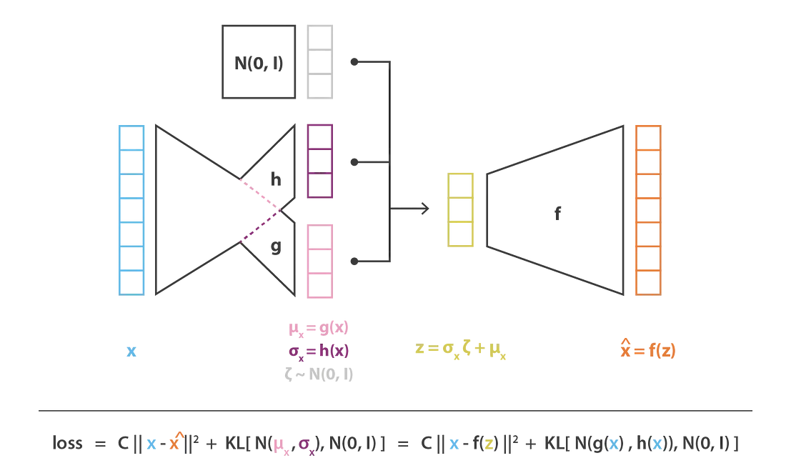
• VAE
  : Evidence $x$로부터 prior $p(z)$를 estimate하는 encoder와 sampling된 $z$로부터 likelihood $p_\theta(x|z)$를 maximize하는 decoder로 구성. Reconstruction loss와 regularization loss로 update.
  

• Diffusion Model
  : Gaussian noise를 추가하는 forward process, denoising U-Net으로 구성된 reverse process. Training은 임의의 timestep $t$에 대해서, sampling은 모든 timestep $T$ ~ $0$에 대해 차례로 denoising 진행.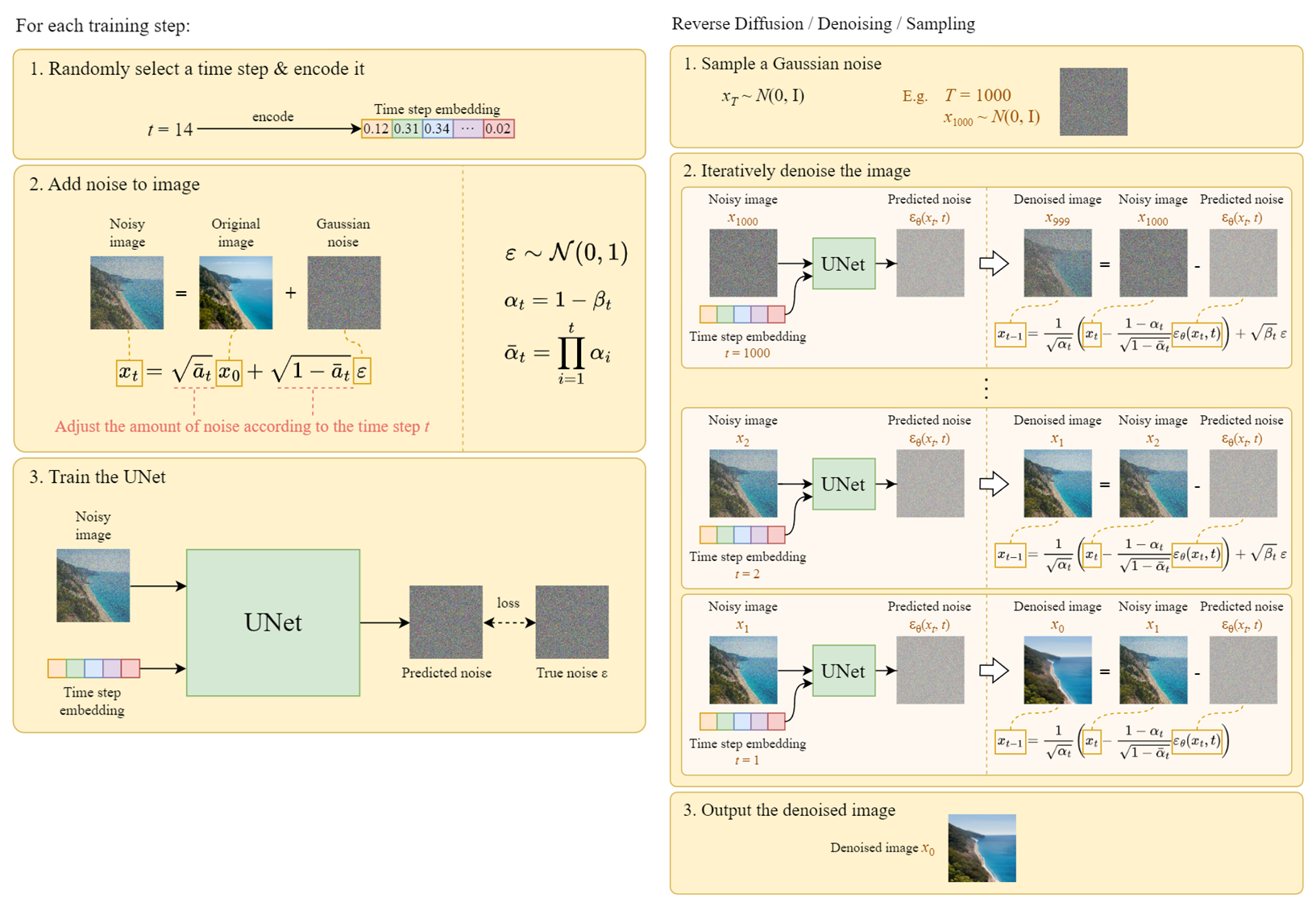

  

  • Samplers
    : https://stable-diffusion-art.com/samplers/

  • Stable Diffusion (Latent Diffusion Model)
    

  • Classifier Guidance
    : Training dataset과 desired class에 대한 pretrained classifier의 gradient $\nabla_{x_t}\log p_\phi(y|x_t)$를 diffusion model에 적용해 desired class로의 sampling을 유도하는 방법.

  • Classifier-Free Guidance
    : Class information을 함께 입력받는 denoising network $\epsilon_\theta(z_\lambda,c)$를 일정 비율로 conditioning을 부여해가며 학습. Sampling 때도 given class와 null class 각각에 대한 noise prediction 값을 interpolate하여 사용. ($w$: Guidance scale, 클수록 condition에 fidelity가 높은 sample 생성)

    $\tilde{\epsilon}_\theta(z_\lambda, c)=(1+w)\epsilon_\theta(z_\lambda,c)-w\epsilon_\theta(z_\lambda)$

  • Instruct-Pix2Pix [InstructPix2Pix: Learning to Follow Image Editing Instructions (Tim Brooks, et al.)]
    $\Rarr$ GPT-3 + Stable Diffusion : Source image, text instruction, Prompt-to-Prompt 모델로 생성된 edited image의 triplet으로 fine-tune.

    *Prompt-to-Prompt
    : Prompt $P$의 개별 textual token이 noisy image $z_t$에 갖는 cross-attention map $M_t$에 집중. 수정된 prompt $P^*$에 대한 $M_t^*$를 word swap, prompt refinement, attention re-weighting의 editing 각각에 알맞게 적용. Source prompt와 target prompt, 고정된 seed 값을 입력받아 두 prompt 각각에 대한 consistent images 생성.

    : Textual description(input caption)과 textual edit(instruction)이 주어지면, GPT-3로 output caption을 생성해낸 후, Prompt-to-Prompt로 각 caption에 대한 image pair 생성.

    $\epsilon_\phi^{w_s, w_y}(x_t;\tilde{x}, y, t)=\epsilon_\phi(x_t;t)+w_s(\epsilon_\phi(x_t;\tilde{x},t)-\epsilon_\phi(x_t;t)) \\\text{ }\text{ }\text{ }\text{ }\text{ }\text{ }\text{ }\text{ }\text{ }\text{ }\text{ }\text{ }\text{ }\text{ }\text{ }\text{ }\text{ }\text{ }\text{ }\text{ }\text{ }\text{ }\text{ }\text{ }\text{ }\text{ }\text{ }\text{ }\text{ }\text{ }\text{ }\text{ }\text{ }\text{ }\text{ }\text{ }\text{ }\text{ }\text{ }\text{ }\text{ }\text{ }\text{ }\text{ }\text{ }\text{ }\text{ }\text{ }\text{ }\text{ }\text{ }\text{ }\text{ }+w_y(\epsilon_\phi(x_t;\tilde{x},y,t)-\epsilon_\phi(x_t;\tilde{x},t))$

• NeRF [NeRF: Representing Scenes as Neural Radiance Fields for View Synthesis (Ben Mildenhall, et al.)]
  https://nuggy875.tistory.com/168
  : 2D screen에서의 각 pixel에 대해(학습 시에는 각 이미지에서 4,096개의 pixel sampling), 카메라의 center of projection을 지나 뻗어나가는 광선을 casting(stratified sampling 사용). 각 광선 상 3D points의 ($x, y, z, \theta, \phi$)를 MLP에 입력하여 얻어낸 ($R, G, B, \sigma$) 값으로 volume rendering(하나의 pixel 값으로 예측).
  : 여러 방향에서의 이미지와 associated camera position으로 학습, 이후 입력으로 넣어주지 않은 random angle에서의 이미지 생성.
  : Volumetric density 및 RGB 값에 대한 INR이라 볼 수 있음 $\rarr$ $\theta$ : Latent parameter, $g$ : Image renderer (MLP), $g(\theta)$: Rendered image

• Score Distillation Sampling (SDS) - [DreamFusion: Text-to-3d using 2d diffusion (Ben Poole, et al.)]
  : NeRF 등의 DIP(Differentiable Image Parametrization)에 대한 학습 방법론. Dream Fields 모델에서의 CLIP(spatial 정보 손실, 주어진 embedding을 만족하는 이미지가 유일하게 정해지지 않아 adversarial sample을 생성하고 학습이 정체될 수 있음)을 pretrained Imagen을 활용해 얻어낸 score function으로 대체.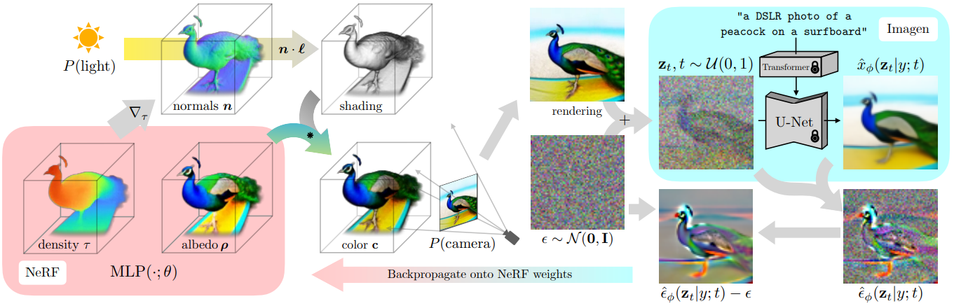

  

  : 기존의 diffusion training loss에서 계산이 어렵고 작은 noise에 대한 conditioning이 어려운 U-Net Jacobian 항을 제거하여 probability density distillation loss gradient 구성.

  

  : SDS와 NeRF-like rendering engine을 사용하여 2D diffusion model을 3D로 전환(3D 혹은 multi-view 학습 데이터 불필요).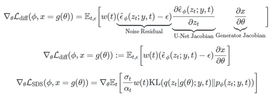

• Stein Variational Gradient Descent (SVGD)

  Variational Inference
  Log marginal likelihood $\ln p(D)=\text{ELBO}+D_{KL}(q(w|\theta)||p(w|D))\ge\text{ELBO}$

  • Likelihood: Parameterized model이 주어진 입출력 데이터를 얼마나 잘 설명할 수 있는가.
  • Posterior: Likelihood를 구하기 위해 필요한 값으로, 주어진 입출력 데이터에 대한 모델 파라미터의 분포 $p(w|D)$. 일반적으로 intractable하여 이를 근사하는 variational 분포 $q(w|\theta)$를 찾는 것이 목표.

  Kernel Methods (http://www.gatsby.ucl.ac.uk/~gretton/coursefiles/lecture4_introToRKHS.pdf)

  • Hilbert Space: Inner product가 정의된 vector space
  • Kernel: Non-empty set $\mathcal{X}=\mathbb{R}^D$와 Hilbert space $\mathcal{H}$에 대해 smooth vector function(feature map) $\phi : \mathcal{X}\rarr\mathcal{H}$와 Hilbert space $\mathcal{H}$의 inner product $<\cdot,\cdot>_\mathcal{H}\text{ }:\text{ }\mathcal{H}\times\mathcal{H}\rarr\mathbb{R}$로 아래와 같이 정의되는 함수 $k : \mathcal{X}\times\mathcal{X}\rarr\mathbb{R}$를 kernel이라 칭함.
    $k(x, x'):=<\phi(x), \phi(x')>_\mathcal{H}$
    : Input(ex. NN parameter)을 Hilbert space에서 정의되는 feature로 mapping 후 inner product 수행.
    : 모든 kernel function은 positive definite함.
  • Reproducing Kernel Hilbert Space (RKHS)
    : $\mathcal{X}\rarr\mathbb{R}$ 로 정의되는 함수들에 대한 space. 각 함수는 input을 feature space로 mapping 후 함수의 파라미터와 inner product하여 $\mathbb{R}$로 mapping.
    $f(x):=<f(\cdot), \phi(x)>_\mathcal{H}=<f(\cdot), k(\cdot,x)>_\mathcal{H} \\\mathcal{H}=\{f:f(x)=\sum_{i=1}^ma_ik(x,x_i), a_i\in\mathbb{R}, m\in\mathbb{N}, x_i\in\mathcal{X}\}$
    : Kernel이 정의되면 RKHS도 정의됨.
  • Stein Discrepancy
    : Stein operator로 smooth vector function $\phi$를 함수 $p$에 대해 바꾸었을 때, 그 값을 함수 $q$에 대해 적분한 값($p$에 대해 적분할 경우 0)으로, 두 함수의 KL-divergence에 대한 derivate에 해당. $\phi$의 종류를 정의하는 function set $\mathcal{F}$가 discriminative power를 결정.
    $\mathbb{D}(q,p)=\max_{\phi\in\mathcal{F}}\{\mathbb{E}_{x\sim q}[\text{Tr}(A_p\phi(x))]\}$
    : $\mathcal{F}$를 RKHS로 정의하면 아래와 같은 closed-form solution을 얻을 수 있고, 이는 앞선 KL-divergence 값을 가장 크게 줄이는 steepest descent 방향에 해당. $\Rarr$ Kernelized Stein Discrepancy(KSD).
    $\mathbb{D}(q,p)=\left|\left|\int_{x\in\mathcal{X}}{[\nabla_x\log p(x)k(x,\cdot)+\nabla_xk(x,\cdot)]q(x)dx}\right|\right|_{\mathcal{H}^d}$

  : $w$ 자체에 대한 분포를 함수의 파라미터를 통해 근사한 기존의 variational inference 방법론과는 달리, $w$와 동일한 차원을 갖는 particle로 얻어지는 empirical distribution이 $w$와 비슷한 분포를 갖도록 유도.

  : 두 분포 사이의 KL-divergence에 대한 gradient는 아래와 같이 정의되는데,

  $E_{q(x)}[f(x)^T\nabla_x\log p(x)+\text{Tr}(\nabla_xf(x))]$

  kernelized Stein discrepancy의 식에 따라 아래의 update method를 가짐.

  $x\larr x-\eta\Delta x, \text{ }\text{ }\Delta x=E_{q(x')}[k(x,x')\nabla_{x'}\log p(x')+\nabla_{x'}k(x, x')], \text{ }\text{ }k(x, x')=\exp(-\frac{1}{h}||x-x'||_2^2)$

  : 직관적으로, particle $x$를 이동시키기 위해 자신을 포함 주변 particle $x'$이 이동해야 하는 방향에 대한 (거리에 반비례하는 kernel 값으로) weighted sum을 활용하며 particle끼리 서로 mode-collapse하지 않도록 update.

---

Questions

Q1. 'Prior'라는 용어가, 특정 modality에 대해 학습된 모델의 능력 혹은 모델이 학습한 데이터의 분포를 포괄적으로 지칭하는 게 맞는지..?
(ex. 'Rich generative prior of text-to-image diffusion models': 미리 학습된 diffusion model이 prompt에서 image를 생성해내는 능력)
$\rarr$ Diffusion model에서 최초의 latent vector를 sampling하는 'prior distribution' (Gaussian)과 서로 헷갈림. 가정으로 두는 분포라는 점에서 둘이 같은 건가..?
$\rarr$ 1-1) 'Distillation'이 다른 modality로 학습된 모델에서 target modality에 유용한 정보(ex. Diffusion model의 estimated score function 값)를 추출(증류)하는 것을 의미하는 건지..?

A1. Prior는 diffusion model architecture 자체가 가지는 capacity 정도로 이해하면 될 듯! Distillation 또한 그 의미가 맞음.

Q2. Original-NeRF가 multi-view 이미지와 카메라 정보를 바탕으로 pixel-wise 지도학습을 진행하는 데에 비해, DreamFusion은 임의의 카메라 각도를 샘플링하여 scratch 상태의 NeRF로 rendering한 후, pre-trained Imagen에 prompt와 noised rendered image를 제공해 score function을 얻어내어 이를 (Imagen으로의 backprop 없이) 학습의 gradient로 활용한다고 이해함. 근데 Imagen이 주어진 prompt에 대해 같은 형태의 object를 반복하여 생성하는가..? 직관적으로 Imagen이 제공하는 score function에 그러한 consistency 조건이 없다면 NeRF의 파라미터는 수렴하지 못하는 것 아닌가..?

A2. 맞음. 따라서 생성 이미지의 diversity를 줄이고 fidelity를 높이기 위해 text guidance scale을 100 정도로 엄청 크게 부여함(일반적으론 7-30 정도로 부여).

Q3. NeRF에선 ($x, y, z, \theta, \phi$)의 정보를 ($R, G, B, \sigma$)로 mapping하는 MLP가 $g$, 그 파라미터가 $\theta$이고, 하나의 3D object에 대해 하나의 파라미터 $\theta$가 matching 되어 input에 따라 multiple sample을 sampling 한다고 이해함. 그렇다면 CSD의 $\{\theta_i\}_{i=1}^N$에 대한 $x^{(i)}=g(\theta_i)$라는 notation이, 예컨대 여러 동물에 대한 이미지를 추출하는 NeRF라고 하면, 각 동물의 종류를 $i$라고 이해하면 되는 건지..? (각 동물에 대한 파라미터가 동물에 대한 underlying feature를 학습)

A3. Text-to-3D의 경우 camera angle에 따른 image $x$를 동일한 $\theta$에 대해 sampling하는 것이 맞음. 하지만 panorama image, video 등에 대한 sampling은 각 patch/frame에 대해 별도의 $\theta_i$가 별도로 학습된다고 생각하면 됨.

Q4. 아래 식에서 kernel $k$는 두 변수가 서로 가까울수록 높은 값을 갖는데 두 번째 항이 의미하는 바는 그럼 repulsive force가 아니라 attractive force 아닌가..?
$x\larr x-\eta\Delta x, \text{ }\text{ }\Delta x=E_{q(x')}[k(x,x')\nabla_{x'}\log p(x')+$$\nabla_{x'}k(x, x')$$], \\\text{ }\text{ }\text{ }\text{ }\text{ }\text{ }\text{ }\text{ }\text{ }\text{ }\text{ }\text{ }\text{ }\text{ }\text{ }\text{ }\text{ }\text{ }\text{ }\text{ }\text{ }\text{ }\text{ }\text{ }\text{ }\text{ }\text{ }\text{ }\text{ }\text{ }\text{ }\text{ }\text{ }\text{ }\text{ }\text{ }\text{ }\text{ }\text{ }\text{ }\text{ }\text{ }\text{ }\text{ }\text{ }\text{ }\text{ }\text{ }\text{ }\text{ }\text{ }\text{ }\text{ }\text{ }\text{ }\text{ }\text{ }\text{ }\text{ }\text{ }\text{ }\text{ }\text{ }\text{ }\text{ }\text{ }\text{ }\text{ }\text{ }\text{ }\text{ }\text{ }\text{ }\text{ }k(x, x')=\exp(-\frac{1}{h}||x-x'||_2^2)$

A4. $\nabla_{x'}\log p(x')$ 앞에 곱해지는 $k(x,x')$ term이 attractive force에 해당.

Q5. Noise prediction term의 baseline function을 기존의 random Gaussian noise $\epsilon$에서 image-conditional noise estimate $\epsilon_\phi^{\omega_s}(\tilde{x}_t^{(i)};\tilde{x},t)$로 수정하여 source image에 대한 detail loss를 줄였다는데 그 논리가 직관적으로 이해가 되지 않음.
아래와 같이 수정된 score function $\Delta\mathcal{E}_t^{(i)}$은 source image에 대한 guidance(fidelity)가 줄어든 것 아닌가..?

$\Delta\mathcal{E}_t^{(i)}=$ $\epsilon_\phi^{\omega_y, \omega_s}(x_t^{(i)};\tilde{x}, y, t)$$-\epsilon_\phi^{\omega_s}(\tilde{x}_t^{(i)};\tilde{x},t)$

$\epsilon_\phi^{\omega_y, \omega_s}(x_t^{(i)};\tilde{x}, y, t)$ $=\epsilon_\phi(x_t;t)+\omega_s($$\epsilon_\phi(x_t;\tilde{x},t)$$-\epsilon_\phi(x_t;t)) \\\text{ }\text{ }\text{ }\text{ }\text{ }\text{ }\text{ }\text{ }\text{ }\text{ }\text{ }\text{ }\text{ }\text{ }\text{ }\text{ }\text{ }\text{ }\text{ }\text{ }\text{ }\text{ }\text{ }\text{ }\text{ }\text{ }\text{ }\text{ }\text{ }\text{ }\text{ }\text{ }\text{ }\text{ }\text{ }\text{ }\text{ }\text{ }\text{ }\text{ }\text{ }\text{ }\text{ }\text{ }\text{ }\text{ }\text{ }+\omega_y(\epsilon_\phi(x_t;\tilde{x},y,t)-\epsilon_\phi(x_t;\tilde{x},t))$

A5. 모델이 textual instruction 정보에 더 중점적으로 학습될 수 있도록 score function의 variance를 조절해 주었다고 이해하면 될 듯.

---

Paper Summary

  Pre-trained diffusion model의 rich prior를 다른 modality에 대한 모델의 학습에 활용하는 SDS(Score Distillation Sampling). 여러 particle이 target distribution을 따르도록 함께 update하는 SVGD(Stein Variational Gradient Descent).

  단일 modality(panorama image, video, 3D scene)의 각 image에 대한 parameter를 SVGD에서의 particle로 두어 서로 consistent하게 학습되도록 유도하는 것이 핵심 아이디어.

  각 modality에 대한 text-guided editing을 위해, pre-trained Instruct-Pix2Pix 모델에서 posterior에 대한 score function을 얻어내 학습에 활용함.

---

What I Learned (or Reviewed)

• Variational Inference, Bayesian Inference
• NeRF, Instruct-NeRF2NeRF
• Diffusion Models: DDPM, DDIM, Stable Diffusion, Samplers, Classifier Guidance, Classifier-Free Guidance (CFG)
• Advanced Diffusion Models: Prompt-to-Prompt, Instruct-Pix2Pix (Score Distillation Sampling)
• Kernel Methods: Reproducing Kernel Hilbert Space (RKHS), Kernelized Stein Discrepancy (KSD), Stein Variational Gradient Descent (SVGD)

---

References

• [논문리뷰] DreamFusion: Text-to-3D using 2D
• [edwith 강연] Stein Variational Gradient Descent