Hi! I'm Jaylnne. ✋

며칠 전 작성한 [ML] 신용카드 사기 거래 탐지 모델 만들어보기 (1) 에서 개선한 내용을 작성한 포스팅입니다. 리스팅해둔 TODO 가 있는데, 이번처럼 (3), (4) 로 작성할 예정입니다.

1. Fix Points

이번 포스팅에 정리해 볼 예정인 fix points 는 아래 세 가지입니다.

• test dataset 은 class imbalance 문제를 유지한 채로 실험하기.
• under sampling 에서 train dataset 의 class 분포를 1:1 이 아닌 2:8 로 해보기.
• classification 결과를 validation accuracy 가 아닌 test accuracy 로 비교하기 (실수 정정)

실제 환경에서 '사기 거래'는 '정상 거래'보다 훨씬 낮은 빈도로 발생할 것입니다. 따라서 test dataset 은 실제의 환경과 유사하도록 극단적인 class imbalance 를 유지한 채 실험을 진행하는 것이 더 적절할 것입니다.

이전 포스팅에서는 under sampling 과정에서 class 의 분포를 1:1로 맞추어주었습니다. 그러나 '사기 거래'에 해당하는 데이터 수가 너무 적어, 너무 많은 '정상 거래' 데이터가 버려진다는 문제가 있었습니다. under sampling 그 자체의 '정보의 소실' 문제를 완전히 해결할 수는 없지만, class 비율을 1:1 이 아닌 2:8 로 실험해봄으로써 버려지는 데이터를 조금 줄여보았습니다.

classification model 들의 성능 비교를 일관성 없이 한 실수가 있었습니다. (validation accuracy 로 했다가, test accuracy 로 했다가...) 코드를 수정하여, 원래의 의도대로 test accuracy 로 모델의 성능을 비교할 수 있도록 했습니다.

2. Scaling

우선, 필요한 라이브러리들을 임포트합니다. 그리고 이전 포스팅에서 진행했던 Amount, Time 변수에 대한 Scaling 을 진행합니다.

import time
import pandas as pd
import numpy as np
import matplotlib.pyplot as plt
from sklearn.preprocessing import RobustScaler
from sklearn.model_selection import train_test_split, GridSearchCV, cross_validate
from sklearn.linear_model import LogisticRegression
from sklearn.neighbors import KNeighborsClassifier
from sklearn.svm import SVC
from sklearn.tree import DecisionTreeClassifier

# Load data
df = pd.read_csv('data/creditcard.csv')

# Scaling
scaler = RobustScaler()

df['scaled_amount'] = scaler.fit_transform(df['Amount'].values.reshape(-1, 1))
df['scaled_time'] = scaler.fit_transform(df['Time'].values.reshape(-1, 1))

df.drop(['Amount', 'Time'], axis=1, inplace=True)

3. test dataset class imbalance 유지

test dataset 에는 class imbalance 를 유지하기로 했습니다. under sampling 을 하기 이전에 train 과 test 를 분리해주면 됩니다.

train, test = train_test_split(df, test_size=0.2, shuffle=True, random_state=42, stratify=df['Class'])

test dataset 의 클래스 분포를 살펴보면 당연히 사기 거래보다 정상 거래의 데이터 수가 훨씬 많은 것을 확인할 수 있습니다.

# Check test dataset class distribution
test_val_cnt = test['Class'].value_counts().reset_index()
plt.bar(test_val_cnt['index'], test_val_cnt['Class'], color=['red', 'blue'], tick_label=['fraud', 'normal'])
plt.title('Class Distribution of test dataset')
plt.show()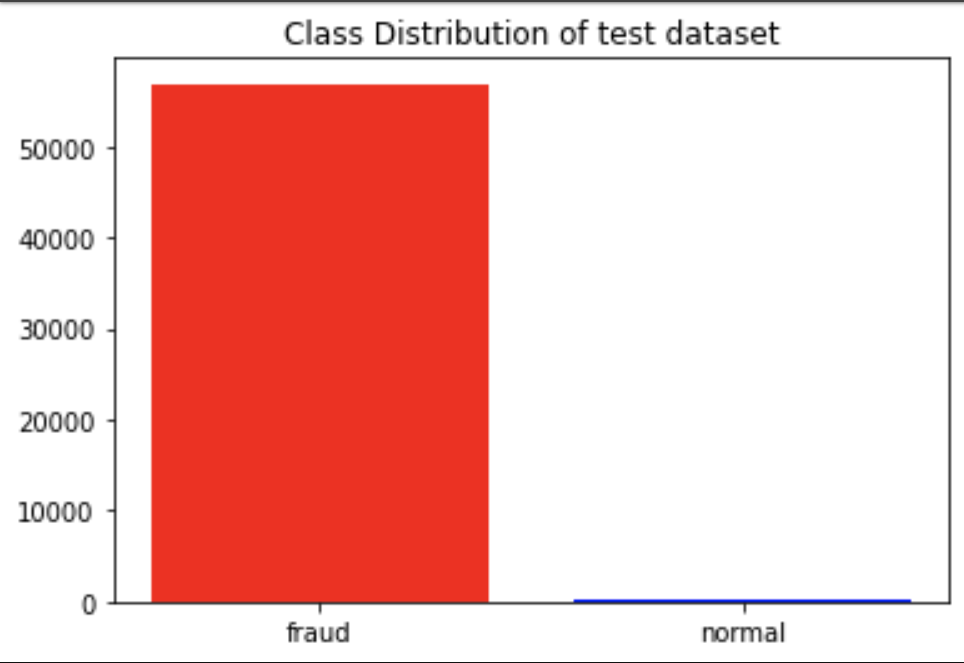

4. Under Sampling

분리한 train dataset 만으로 under sampling 을 진행합니다.

# Under Sampling train dataset
fraud = train[train['Class']==1].reset_index(drop=True)
normal = train[train['Class']==0]

num_of_normal = len(fraud) * 4    # 2:8 비율

normal = normal.sample(n=num_of_normal, random_state=42, ignore_index=True)

print(f'Length of fraud data: {len(fraud)}')
print(f'Length of normal data: {len(normal)}')

train = pd.concat([fraud, normal], ignore_index=True)

# output
Length of fraud data: 394
Length of normal data: 1576

5. Train Classifiers

이전 포스팅과 같이, Logistic Regression, K-Neighbors, SVC, Decision Tree 4 가지 분류 모델을 학습시켜보겠습니다. 대신, 이전과 달리 성능은 test accuracy 로 비교합니다.

# Train Classifier
X_train = train.drop('Class', axis=1)
y_train = train['Class']
X_test = test.drop('Class', axis=1)
y_test = test['Class']

model = LogisticRegression(max_iter=10000)
params = {'penalty':['l2'], 'C':[0.001, 0.01, 0.1, 1, 10, 100, 1000]}
grid = GridSearchCV(model, params, scoring=['accuracy', 'roc_auc'], refit='roc_auc', return_train_score=True, cv=5)
grid.fit(X_train, y_train)

print('< Logistic Regression Results >')
print(f'Total fit time: {grid.cv_results_["mean_fit_time"].sum()}')
print(f'The best params: {grid.best_params_}')
print(f'Test accuracy: {round(grid.score(X_test, y_test) * 100, 2)}%')
print('\n')

model = KNeighborsClassifier()
params = {"n_neighbors": list(range(2,5,1)), 'algorithm': ['auto', 'ball_tree', 'kd_tree', 'brute']}
grid = GridSearchCV(model, params, scoring=['accuracy', 'roc_auc'], refit='roc_auc', return_train_score=True, cv=5)
grid.fit(X_train, y_train)

print('< K-Neighbors Results >')
print(f'Total fit time: {grid.cv_results_["mean_fit_time"].sum()}')
print(f'The best params: {grid.best_params_}')
print(f'Test accuracy: {round(grid.score(X_test, y_test) * 100, 2)}%')
print('\n')

model = SVC()
params = {'C': [0.5, 0.7, 0.9, 1], 'kernel': ['rbf', 'poly', 'sigmoid', 'linear']}
grid = GridSearchCV(model, params, scoring=['accuracy', 'roc_auc'], refit='roc_auc', return_train_score=True, cv=5)
grid.fit(X_train, y_train)

print('< SVC Results >')
print(f'Total fit time: {grid.cv_results_["mean_fit_time"].sum()}')
print(f'The best params: {grid.best_params_}')
print(f'Test accuracy: {round(grid.score(X_test, y_test) * 100, 2)}%')
print('\n')

model = DecisionTreeClassifier()
params = {
    "criterion": ["gini", "entropy"], 
    "max_depth": list(range(2,10,1)), 
    "min_samples_leaf": list(range(2,10,1))
}
grid = GridSearchCV(model, params, scoring=['accuracy', 'roc_auc'], refit='roc_auc', return_train_score=True, cv=5)
grid.fit(X_train, y_train)

print('< Decision Tree Results >')
print(f'Total fit time: {grid.cv_results_["mean_fit_time"].sum()}')
print(f'The best params: {grid.best_params_}')
print(f'Test accuracy: {round(grid.score(X_test, y_test) * 100, 2)}%')
print('\n')

< Logistic Regression Results >
Total fit time: 0.18196382522583007
The best params: {'C': 0.01, 'penalty': 'l2'}
Test accuracy: 97.69%


< K-Neighbors Results >
Total fit time: 0.023036813735961916
The best params: {'algorithm': 'auto', 'n_neighbors': 4}
Test accuracy: 95.92%


< SVC Results >
Total fit time: 0.27288045883178713
The best params: {'C': 1, 'kernel': 'rbf'}
Test accuracy: 97.6%


< Decision Tree Results >
Total fit time: 2.1222315311431887
The best params: {'criterion': 'entropy', 'max_depth': 5, 'min_samples_leaf': 9}
Test accuracy: 94.85%

6. Next to do

다음 포스팅에서는 다음 2 가지 fix points 를 다루어보고자 합니다.

• 오토인코더(Autoencoder)를 활용하여 Anomaly Detection 문제에 접근
• 피어슨 상관계수가 아닌 다른 방식으로 Feature Selection