1. Linear Regression

The most common method for fitting a regression line is the method of least-squares.

This method calculates the best-fitting line for the observed data by minimizing the sum of the squares of the vertical deviations from each data point to the line (if a point lies on the fitted line exactly, then its vertical deviation is 0).

Because the deviations are first squared, then summed, there are no cancellations between positive and negative values.

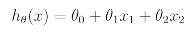
Parameters( 혹은 weight라고도 불림)를 이용하여 X -> Y로 선형 함수를 Mapping하는 방식이다.

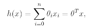
이를 일반화하면 다음과 같은 식을 도출할 수 있다.

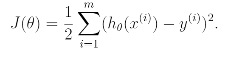
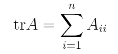
Parameters 각각의 값을 구하기 위해 cost function을 다음과 같이 정의한다.

---

2. LMS Algorithm

We want to choose parameter so as to minimize J. To do so let's use a search algorithm that starts with some "initial guess" for parameter.

And that repeatedly changes parameter to make J smaller until hopefully we converge to a value of parameter that minimizes J.

Gradient Descent Algorithm은 다음과 같다.

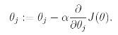
여기서 Alpha는 Learning Rate라고 불리며 이를 J에 대한 식으로 나타내면 다음과 같다.

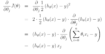
The rule is called the LMS update rule and is also known as the Widrow-Hoff learning rule. This rule has several properties that seem natural and intuitive.
For instance the magnitude of the update is proportional to the error term.

LMS update rule은 다음과 같이 표현할 수 있다.

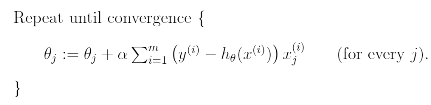
This is simply gradient descent on the original cost function J. And is also called batch gradient descent.

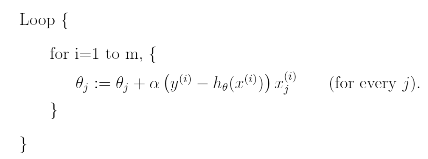
In this algorithm, we repeatedly run through the training set, and each time we encounter a training example, we update the parameters according to the gradient of error with respect to that single training example only. This algorithm is called stochastic gradient descent( or incremental gradient descent).

---

3. The normal equations

Gradient Descent gives one way of minimizing J.
Let's discuss second way. This time performing the minimization explicitly and without resorting to an iterative algorithm.

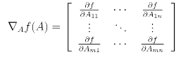
2.1 Matrix Derivatives

We can mapping from n-by-n matrices to the real numbers

We also introduce trace operator written "tr".

trace means sum of diagonals. So there are several properties we can use.

(1) trABC = trBAC = trBCA
(2) trA = inverse(trA)
(3) tr(A+B) = trA + trB
(4) tr(aA) = atrA

Also we can use these properties too.

2.2 Least squares revisited

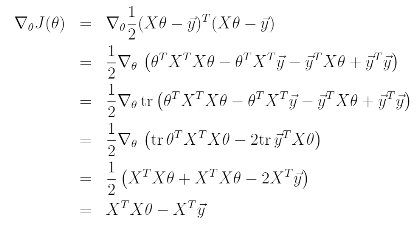
Armed with the tools of matrix derivatives, let us now proceed to find in closed-form the value of theta that minimizes J.

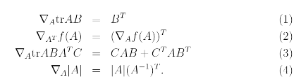
위의 식을 도출하기 위해 필요한 성질은 다음과 같다.

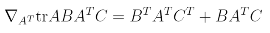
AT = theta, B = BT = XTX, C=1을 대입하여 계산하여 구할 수 있다.

To be continued...