.png)
1. Generative Learning Algorithms
Consider a classification problem in which we want to learn to distinguish between elemphants(y=1) and dogs(y=0), based on some features of an animal.
Given training set, an algorithm like logistic regression or the perceptron algorithm tries to find a straight line -that is a decision boundary- that separates the elephants and dogs.
Then to classify a new animal as either an elephant or a dog, it checks on which side of the decision boundary if falls, and makes its prediction accordingly.
But here's a different approach. First looking at elephant we can build a model of what elephants look like. Then looking at dogs we can build a seperate model of what dogs look like. Finally to classify a new animal, we can match the new animal against the elephant model and match it against the dog model, to see whether the new animal looks more like the elephants or more like the dogs we had seen it the training set.
위의 예시에서 알 수 있듯이 Logistic regression이나 Perceptron algorithm은 p(y|x)를 바로 학습하고자 하거나 input을 0~1 상에 바로 표현하고자 한다. 우리는 이러한 알고리즘을 Discriminative Learning Algorithm이라 부른다.
다만 두번째 방식과 같이 p(x|y)나 p(y) 모델을 시도하는 알고리즘을 Generative Learning Algorithm이라 부른다.
위의 예시에서 살펴보면 p(x|y=0)은 dog의 특징을 가진 분포에 대한 모델이며, p(x|y=1)은 elephant의 특징을 가진 분포에 대한 모델이라고 할 수 있다.
2. Bayes Rule
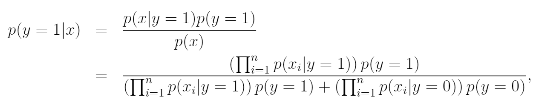
After modeling p(y) and p(x|y), our algorithm can then use Bayes rule to derive the posterior distribution on y given x:
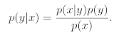
The denominator is given by
and thus can also be expressed in terms of the quantities p(x|y) and p(y) that we've learned.
3. Gausian Discriminant Analysis
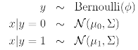
When we have a classification problem in which the input features x are continuous-valued random variables, we can then use Gaussian Discriminant Analysis (GDA) model, which models p(x|y) using a multivariate normal distribution.
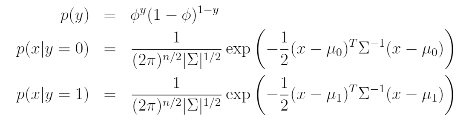
The model is :
Writing out the distribution, this is :
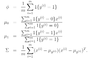
We find the maximum likelihood estimate of the parameters to be :
Pictorially, what the algorithm is doing can be seen in as follows:
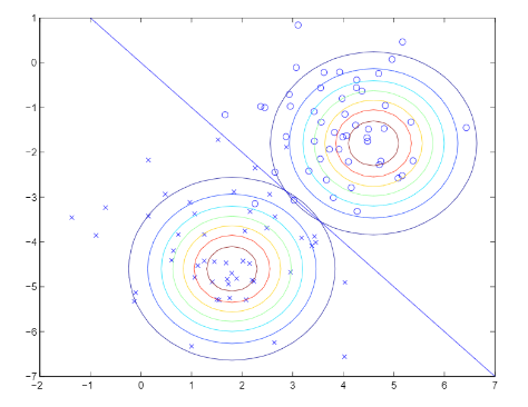
From the picture above, note hat the two Gaussians have contours that are the same shape and orientation, since they share a covariance matrix, but they have different means u0, u1.
추가적으로 위의 그림에서 직선은 p(y=1|x)=0.5에 대한 decision boundary를 제공해주며, 해당 boundary의 한 부분에서는 y=1이 나올 가능성이 높으며, 나머지 부분에서는 y=0으로 예상될 것이다.
4. Naive Bayes
To model p(x|y), we will therefore make a very strong assumption. We will assume that the x's are conditionally independent given y. This assumption is called the Naive Bayes assumption, and the resulting algorithm is called the Naive Bayes classifier.
Naive Bayes에서 "Naive"라는 형용사가 붙은 이유는 분류를 쉽고 빠르게 하기 위해 classifier에 사용하는 변수들이 서로 "확률적으로 독립"이라는 다소 순진하고 억지스러운 가정을 했기 때문이다. feature가 많은 경우 연관 관계를 모두 고려하기보다 단순화하여 쉽고 빠르게 판단을 내릴 때 주로 사용되지만, 확률적으로 독립이라는 가정에 위배되는 경우 에러가 발생할 수 있기 때문에 주의가 필요하다.
Naive Bayes는 multi-class classification에서 쉽고 빠르게 예측이 가능하며, 변수가 독립이라는 가정이 유효하다면 logistic regression과 같은 방식에 비해 훨씬 결과가 좋고 학습 데이터가 적게 필요하다는 장점이 있다.
다만, 학습 데이터에는 없지만 검사 데이터에는 존재하는 category에서는 확률이 0이 되어 정상적인 예측이 불가능하며, 독립이라는 가정이 성립하지 않는다면 결과에 에러가 발생할 수 있다는 단점이 있다.
5. Laplace Smoothing
There is problem in Naive Bayes that it is statistically a bad idea to estimate the probability of som event to be zero just because you haven't seen it before in your finite training set.
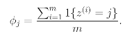
Take the problem of estimating the mean of a multinomial random variable z taking valures in {1,2,...,k}. We can parameterize our multinomial with p(z=i). Given a set of m independent observations {z(1), ..., z(m)}, the maximum likelihood estimates are given by
As we saw previously, if we were to use these maximum likelihood esimates, then some of the pi's might end up as zero, which was a problem. To avoid this, we can use Laplace Smoothing which replaces the above estimate with
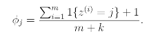
Here we added 1 to the numerator and k to the denominator.
만약 새로 가져온 데이터에 새로운 값이 등장했다면(training set에서 보지 못한 data의 등장) training set을 통해 계산된 확률은 0이 된다. 이렇게 training data에 최적화 되어 새로운 data를 잘 분류하지 못하는 overfitting 문제를 해결하기 위한 방법이 Laplace Smoothing이다.
원래 확률이 0이 될 feature에 어떤 값을 더해주어 전체를 0으로 만드는 불상사를 방지하며, 더해지는 k 값에 따라 smoothing의 정도가 달라지게 된다.
강의 링크 : Stanford CSS229 Youtube
To be continued...