.png)
Support Vector Machine은 Decision Boundary, 즉 분류를 위한 기준선을 정의하는 모델이다. 분류되지 않은 새로운 점이 나타날 때 경계의 어느 쪽에 속하는지 확인하여 분류 과제를 수행하게 함이 목적이다.
Margin은 결정 경계와 서포트 벡터 사이의 거리를 의미한다. 최적의 결정 경계는 마진을 최대화하며 n개의 속성을 가진 데이터에는 최소 n+1개의 서포트 벡터가 존재한다. SVM에서 결정 경계를 정의하는 것이 결국 서포트 벡터이기 때문에 데이터 포인트 중에서 서포트 벡터만 잘 골라내면 나머지 수많은 데이터 포인트들을 무시할 수 있기에 매우 빠르다는 장점이 있다.
1. Margins : Intuition
For a different type of intuition, consider the following figure, in which x's represent positive training examples, o's denote negative training examples, a decision boundary is also shown and three points have also been labeled A,B,C.
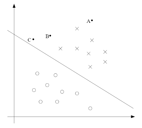
Notice that the point A is very far from the decision boundary. If we are asked to make a prediction for the value of y at A, it seems we should be quite confident that y=1 there. Conversely, the point C is very close to the decision boundary, and while it's on the side of the decision boundary on which we would predict y=1, it seems likely that just a small change to the decision boundary could easily have caused our prediction to be y=0.
Hence we're much more confident about our prediction at A than C. The point B likes in-between these two cases and more broadly, we see that if a point is far from the seperating hyperplane, than we may be significantly more confident in our prediction.
위의 설명에서 알 수 있듯이 Margin은 decision boundary와 support vector 사이의 거리로서 A가 C보다 decision boundary에서의 거리가 멀기 때문에 y=1이라는 prediction에 더 큰 확신을 가질 수 있으며, 가장 가까운 C까지의 거리가 Margin이 될 것이다.
2. Notation
To make our discussion of SVM easier, we'll first need to introduce a new notation for talking about classification. We will be considering a linear classifier for a binary classification problem with labels y and features x.
From now on we'll use y - {-1,1} instead {0,1} to denote the class labels.
Also, rather than parameterizing our linear classifier with the vector theta, we will use parameter w, b and write our classifier as
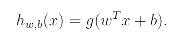
Here g(z)=1 if z>=0 and g(z)=-1 otherwise. This w,b notation allows us to explicitly treat the intercept term b separately from the other parameters. Thus b takes the role of what was prerviously theta0 and w takes the role of inverse[theta(0-n)].
Note that our classifier will directly predict either -1 or 1, without first going through the intermediate step of estimating the probability of y being 1.
SVM에서는 theta를 파라미터로 사용하는 것이 아니라 w와 b를 파라미터로 사용한다. b는 이전에 theta0가 수행하던 역할을 맡았으며, w는 이전에 theta0부터 n까지의 벡터의 inverse vector가 수행하던 역할을 맡게 된다.
3. Functional and geometric margins
(1) Functional Margin
Now Let's formalize the notions of the functional and geometric margins. Given a training example(x(i), y(i)), we define the functional margin of (w,b) with respect to the training example
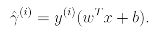
Note that if y(i)=1, then for the functional margin to be large, we need wTx+b to be large positive number.
Conversely if y(i)=-1, then for the functional margin to be large, we need wTx+b to be a large negative number. Moreover if y(i)(wTx+b) > 0, then our prediction on this example is correct. Hence a large functional margin represents a confident and a correct prediction.
Given a training set S = {(x(i), y(i); i=1,...,m}, we also define the function margin of (w,b) with respect to S to be the smallest of the functional margins of the individual training examples.
(2) Geometric Margin
Consider the picture below:
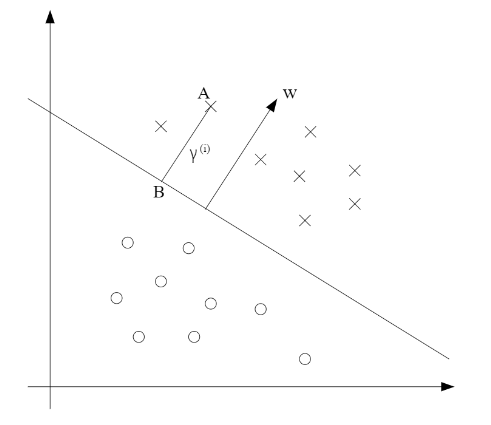
The decision boundary corresponding to (w,b) is shown, along with the vector w. Note that w is orthogonal(at 90 degree) to the separating hyperplane. Consider the point at A, which represents the input x(i) of some training example with label y(i) = 1. Its distance to the decision boundary is given by the line segment AB.
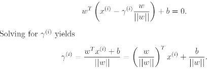
To find the value of distance we use unit-length vector w/||w|| which pointing in the same direction as w. Also all points x on the decision boundary satisfy the equation wTx+b = 0. Hence :
4. The optimal margin classifier
Since multiplying w and b by some constant results in the functional margin being multiplied by that same constant, this is indeed a scaling constraint, and can be satisfied by recaling w,b. Plugging this into our problem above, and noting that maximizing 1/||w|| is the same thing as minimizing ||w||^2, we now have the following optimization problem:
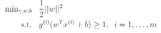
We've now transformed the problem into a form that can be efficiently solved. The above is an optimization problem with a convex quadratic objective and only linear constraints. Its solution gives us the optimal margin classifier. This optimization problem can be solved using commercial quadratic programming code.
5. Lagrange duality
Let's discuss about solving constrained optimization problems. We use method of Lagrange multipliers to solve it. And in this method, we define the Lagrangisan to be
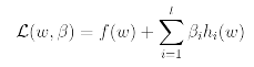
Here the beta's are called the Lagrange multipliers. We would then find and set L's partial derivatives to zero and solve for w and beta.
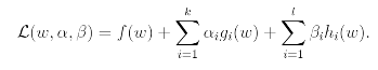
Now we will generalize this to constrained optimization problems in which we may have inequality as well as equality constraints. Due to time ocnstraints, we won't really be able to do the theory of lagrange duality justice. we will then apply to our optimal margin classifier's optimization problem.
Recall primal optimization problem and to solve it we start by defining the generalized Lagrangian:
Under assumptions, there must exist w, alpha, beta so that w is the solution to the primal problem, alpha, beta are the solution to the dual problem, and moreover p=dL(w, alpha, beta). Moreover w, alpha, beta satisfy the Karush-Kuhn-Tucker (KKT) conditions which are as follows:
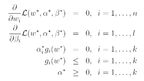
Overall, SVM has only a small number of "support vectors"; the KKT dual complementarity condition will also give us our convergence test when we talk about the SMO algorithm.
6. Optimal margin classifiers
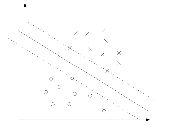
The points with the smallest margins are exactly the ones closet to the decision boundary; Here these are the three points that lie on the dashed lines parallel to the decision boundary.
Thus, only three of the alpha's will be non-zero at the optimal solution to our optimization problem. These three points are called the support vectors in this problem.
강의 링크 : Stanford CS229 Youtube
TO BE CONTINUED...