Title

NeRF: Representing Scenes as Neural Radiance Fields for View Synthesis (ECCV 2020, Oral)

Abstract

• SOTA for synthesizing novel views of complex scenes
• Optimize an underlying continuous volumetric scene function with sparse set of input views
• Fully-connected deep network
  - Input: single continuous 5D coordinate (spatial location $(x,y,z)$ & viewing direction$(\theta, \phi)$)
  • Output: volume density & view-dependant emitted radiance at that spatial location
• Querying 5D coordinates along camera rays & classic volume rendering techniques => Project the output colors and densities into an image => synthesize views
• Volume rendering is naturally differentiable -> only input required to optimize representation is a set of images with known camera poses
• Describe how to effectively optimize neural radiance fields
  - render photorealistic novel views of scenes
  • results that outputperform prior work on neural rendering and view synthesis
• Urge readers to view supplementary video for synthesis results

1 Introduction

we address the long-standing problem of view synthesis in a new way by directly optimizing parameters of a continuous 5D scene representation to minimize the error of rendering a set of captured images.

NeRF

• Represent a static scene as a continuous 5D function
• Function outputs
  - radiance emitted in each direction $(\theta, \phi)$ at each $(x, y, z)$ point in space
  - Density at each point (differential opacity controlling how much radiance is accumulated by a ray passing through $(x, y, z)$
• Optimizes a deep fully-connected neural network (MLP)
  - Regressing from a single 5D coordinate $(x, y, z, \theta, \phi)$ to a single volume density and view-dependant RGB color
• Neural radiance field (NeRF) of a particular viewpoint
• To render NeRF,
  - March camera rays through the scene -> sampled set of 3D points
  • Those points and their corresponding 2D viewing directions -> NN -> set of colors and densities
  • Colors and densities -> classical volume rendering -> accumulate those into a 2D image
• The process is naturally differentiable -> gradient descent to optimize the model
• Minimizing the error between each observed image and the corresponding views rendered from the representation.
  => Coherent model of the scene by assigning high volume densities and accurate colors to the locations that contain the true underlying scene content.
  

Additional Method

• Basic implementation of optimizing NeRF -> does not converge to a high-resolution & inefficient in the required number of samples per camera ray
• Transform input 5D coordinates with a positional encoding -> MLP represents higher frequency scene representation.

Pros of NeRF

• Volumetric representation
  • complex real-world geometry & gradient-based optimization
• Overcomes prohibitive storage costs of discretized voxel grids

Technical contributions

1. 5D neural radiance field(basic MLP networks) that represents complex scenes
2. Differentiable rendering based on classical volume rendering techniques.(hierarchical sampling strategy)
3. Positional encoding to map 5D input into a high-dim space

2. Related Work

Quick 3D vision terms

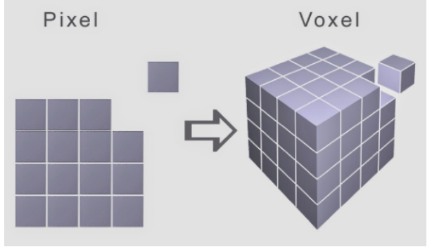
• Voxel grid

Representing objects in the weights of an MLP

• 3D spatial location to an implicit representation of the shape. => unable to produce realistic scenes.

Neural 3D shape representations

• xyz coordinate -> signed distance / occupancy fields

Signed Distance Field

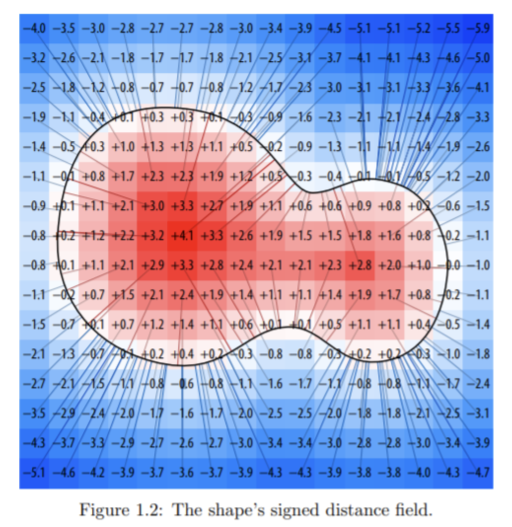
• signed distance field represents geometry with distance from the object's surface.

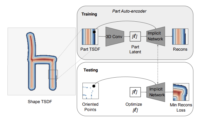
• TSDF shape for representing 3d mesh.

Occupancy fields

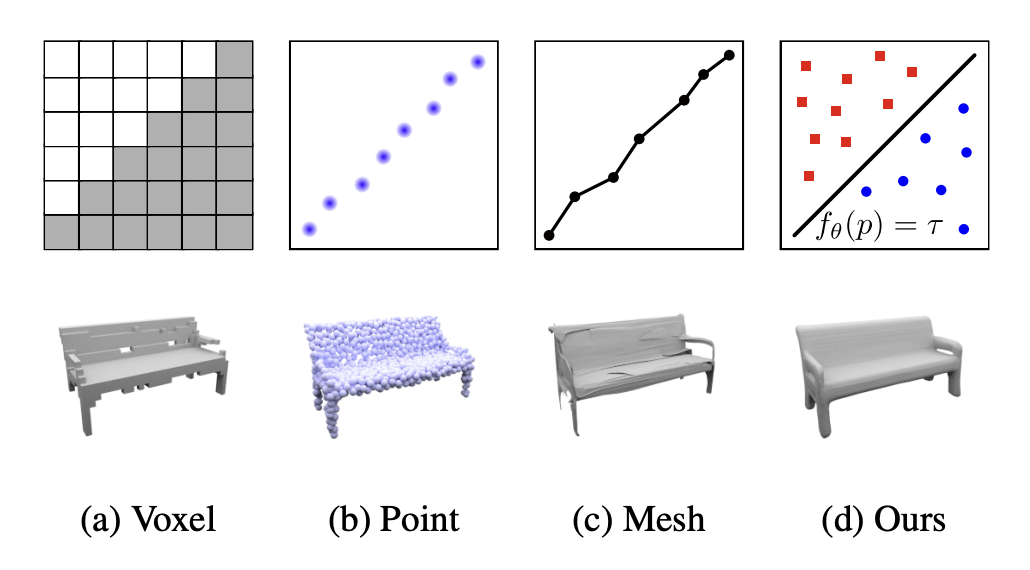
• Continuous decision boundary of a classifier(DNN) as a 3D surface

Limitation

• Limited by their requirement of access to ground truth 3D geometry
• Limited to simple shapes with low geometric complexity -> oversmoothed renderings.

View synthesis and image-based rendering

Case for Dense sampling

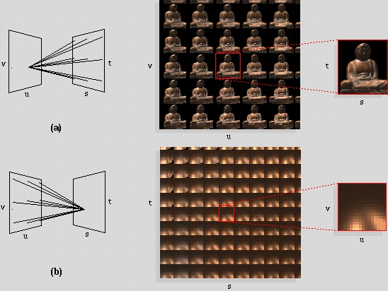
• photorealistic novel view can be reconstructed by simple light field sample interpolation
  

• Figure of light field rendering (1996)

Case for sparser view sampling

• Prediction with traditional geometry and appearance representation

Mesh-based representations of scenes

• Large-Scale texturing of 3D reconstruction (2014) -> diffuse based

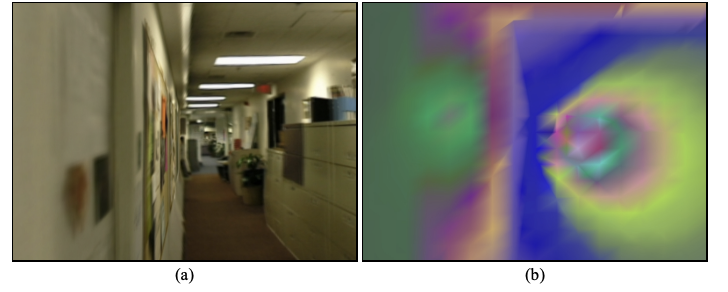
• blending field with view-dependant representation (2001)

Gradient descent based mesh optimizations

• Differentiable rasterizers
  

  • $I_i=w_0u_0+w_1u_1+w_2u_2$
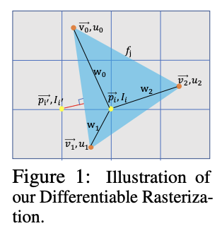
  • Approximate gradients with respect to pixel positions using first-order Taylor approximation

• Pathtracers

=> Gradient-based mesh optimization based on image reprojection is often difficult (local minima or poor conditioning of the loss landscape) + requires fixed topology -> unavailable for real-world scene.

Volumetric representations

• Set of input RGB images -> high-quality photorealistic view synthesis

• early volumetric approaches (observed image -> direct prediction of color voxel grids)

• Large datasets of multiple scene -> DNN that predict sampled volumetric representation

• CNN to represent voxel grids

=> Voxel based approaches are limted by poor time and space complexity (discrete sampling)

3. Neural Radiance Field Scene Representation

• Continuous scene as a 5D vector-valued function
• Input : 3D location $\mathbf{x}=(x,y,z)$ + 2D viewing direction $(\theta, \phi)$
• Output: emitted color $\mathbf{c}=(r, g, b)$ & volume density $\sigma$.
• Approximate continuous 5D scene representation with an MLP network $F_{\theta}:(\mathbf{x}, \mathbf{d})\rightarrow (\mathbf{c}, \sigma)$
• Network predicts volume density $\sigma$ as only a function of location $\mathbf{x}$ (encourge the representation to be multiview consistent)

Network structure

• MLP $F_\theta$

  • $\mathbf{x}$ -> 8 fully-connected layer(ReLU, 256 channel) -> $\sigma$, 256-dim feature vector
  • feature vector $\oplus$ viewing direction -> 1 full layer(ReLU, 128 channel) -> $\mathbf{c}$

  

4. Volume Rendering with Radiance Fields

Volume Rendering

• NeRF render the color of any ray passing through a scene using principles from classical volume rendering
• Volume density $\sigma(\mathbf{x})$ -> differential probability of a ray terminating at an infinitesimal particle at location $\mathbf{x}$.
• Expected color $C(\mathbf{r})$ of camera ray $\mathbf{r}(t)=\mathbf{o}+t\mathbf{d}$:
  • $C(\mathbf{r})=\int_{t_n}^{t_f}T(t)\sigma(\mathbf{r}(t))\mathbf{c}(\mathbf{r}(t), \mathbf{d})dt$
  • $t_n, t_f$ are near and far bounds
  • $T(t)=exp(- \int_{t_n}^{t}\sigma(\mathbf{r}(s))ds)$ -> accumulated transmittance along the ray
    - Probability that the ray travels from $t_n$ to $t$ without hitting any other particle.

Estimating integral

• Estimate continuous integral with quadrature(구적법).

• Stratified sampling(<-> deterministic quadrature of voxel grid rendering)

  • Partition $[t_n, t_f]$ into $N$ evenly-spaced bins
  • draw one sample uniformly at random from each bin
  • $t_i \sim U\left[t_n + {i-1\over N}(t_f-t_n), t_n+{i\over N}(t_f-t_n) \right]$

• Use the samples to estimate $C(\mathbf{r})$ with quadrature rule

  • $\hat{C}(\mathbf{r})=\sum^{N}_{i=1} T_i(1-\exp(-\sigma_i\delta_i))\mathbf{c}_i$
  • $\text{where }T_i=\exp(-\sum_{j=1}^{i-1}\sigma_j\delta_j)$
  • $\delta_i=t_{i+1}-t_i$: distance between adjacent samples

• $\hat{C}(\mathbf{r})$ is trivially differentiable and reduces to traditional alpha compositing with $\alpha_i = 1-\exp(-\sigma_i\delta_i)$.

5. Optimizing a Neural Radiance Field

• Above components are not sufficient for state-of-the-art quality

• 2 improvements

  • Positional encoding of the input coordinates
  • Hierarchical sample -> efficiently sample high-frequency representation

  

5.1 Positional Encoding

• Deep networks are biased towards learning lower frequency functions. -> perform poorly at high-frequency variation in color and geometry.
• Mapping inputs to a high dim space using high frequency functions enables better fitting of data that contains high frequency variation.
• $F_\theta=F'_\theta \circ\gamma$
  • $\gamma$ is not learnable.
  • $\gamma$ is a mapping from $\mathbb{R}$ into a higher dim $\mathbb{R}^{2L}$
  • $\gamma(p)=(\sin(2^0\pi p), \cos(2^0\pi p), \cdots, \sin(2^{L-1}\pi p), \cos(2^{L-1}\pi p))$
  • $\gamma$ is applied separately to each of the 3 coordinate in $\mathbf{x}$, and to 3 components of the Cartesian viewing direction unit vector $\mathbf{d}$ ($\mathbf{d}$ is equivalent with $(\theta, \phi)$
  • $L=10$ for $\gamma(\mathbf{x})$ and $L=4$ for $\gamma(\mathbf{d})$.

Difference with PE in Transformer

PE in transformer

• Provide discrete positions of tokens in a sequence
• Used for providing position information to architecture that does not contain any notion of order

PE in NeRF

• Fuctions to map continuous input coordinates into a high dim space
• Enable MLP to more easily approximate a higher frequency function

5.2 Hierarchical volume sampling

• Inefficient rendering strategy (evaluate at $N$ query points along camera ray)
  • free space and occluded regions do not contribute to output.
• Hierarchical representation -> allocating samples proportionally to their expected effect on the final rendering => increases rendering efficiency

Network

• Optimize two network to represent the scene
• "coarse" and "fine"

1. sample $N_c$ locations using stratified sampling
2. evaluate "coarse" network at these locations
3. Use output of "coarse" network to produce more informed sampling of points along each ray where samples are biased towards the relevant parts of the volume.
   • Rewrite alpha composited color from the coarse network $\hat{C}_c(\mathbf{r})$ as a weighted sum of all sampled colors $c_i$ along the ray.
   • $\hat{C}_c(\mathbf{r})=\sum_{i=1}^{N_c}w_ic_i$ ($w_i=T_i(1-\exp(-\sigma_i\delta_i))$)
   • Normalize the weights as $\hat{w}_i={w_i \over \sum_{j=1}^{N_c} w_j}$ => piecewise-constant PDF along the ray
4. Sample a second set of $N_f$ locations from the distribution with inverse transform sampling
5. Evaluate "fine" network at the union of the first and second set of samples
6. Compute the final rendered color of the ray $\hat{C}_f(\mathbf{r})$ using Eqn.3 but using all $N_c+N_f$ samples.

=> Allocates more samples to regions we expect to contain visible content.

5.3 Implementation details

• Each scene optimization requires
  • dataset of captured RGB images of the scene
  • corresponding camera poses and intrinsic parameter + scene bounds
    • estimated from COLMAP structure-from motion package
• At each optimization iteration,
  1. randomly sample a batch of camera rays from the set of all pixels in the dataset
  2. hierarchical sampling -> query $N_c$ samples from coarse network and $N_c + N_f$ samples from fine network
  3. Volume rendering -> render the color of each ray from both sets of samples
  4. Loss calculation (total squared error between rendered and true pixel colors)
  • $\mathcal{L}=\sum_{\mathbf{r}\in\mathcal{R}} [{\|\hat{C}_c(\mathbf{r})-C(\mathbf{r})\|}^2_2+{\|\hat{C}_f(\mathbf{r})-C(\mathbf{r})\|}^2_2]$
    • $\mathcal{R}$ -> set of rays in each batch

5. Final rendering with only $\hat{C}_f(\mathbf{r})$

• Details
  • Batch size: 4096
  • $N_c=64$, $N_f=128$
  • Adam (weight decay of $5\times 10^{-4}$ to $5\times10^{-5})$
  • Single scene optimization: 100-300k iteration (1-2 day in single V100)

6. Results

6.1 + 6.2 Datasets and Comparisons

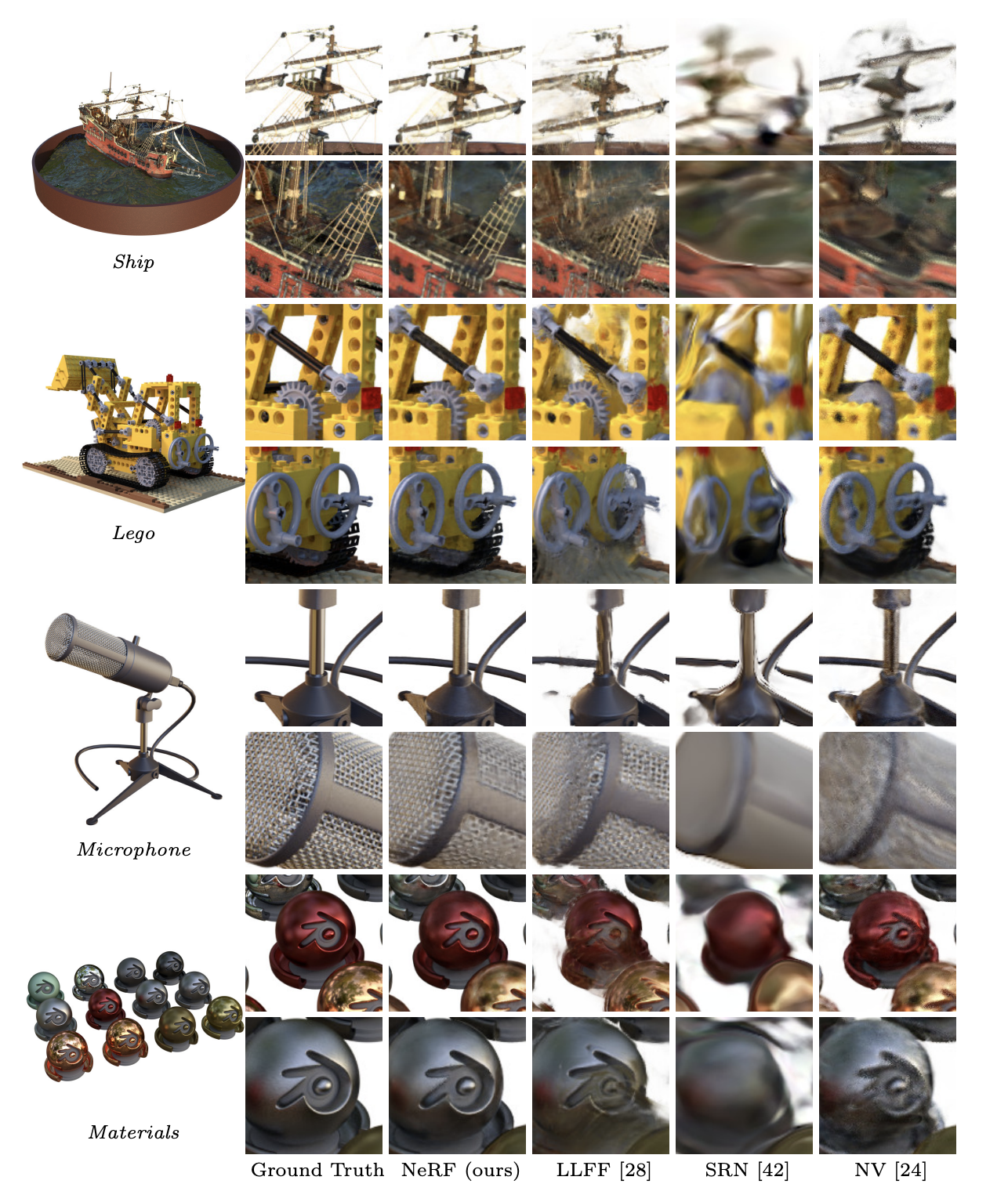
Comparison on synthetic datset with physically-based renderer

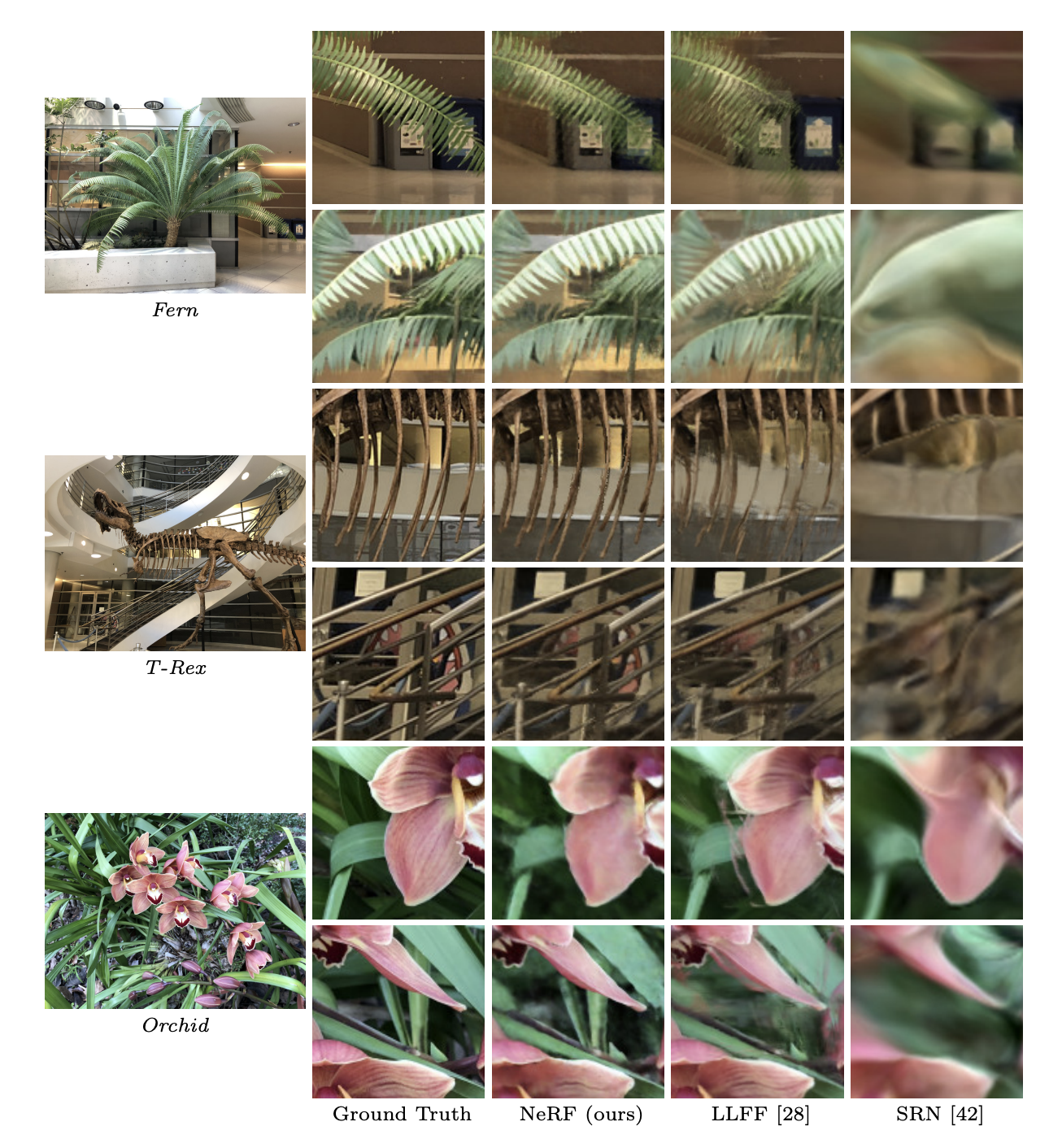
Comparisons on real world scenes

6.3 Discussion

• NeRF outperform both baselines
  • SRN: heavily smoothed geometry and texture & limited by single depth and color per camera ray
  • NV: While can capture detailed geometry and appearance, fails at scaling for find detail in high resoultion (due to underlying explicit $128^3$ voxel grid
  • LLFF: frequently fails to estimate correct geometry in synthetic datasets(due to limited sampling guide line of 64 pixels)

Time vs space tradeoffs

• All single scene methods take at least 12 hours to train per scene except LLFF(10 minutes and under)
• LLFF requires 15GB for every input image
• NeRF: 5MB for network weights

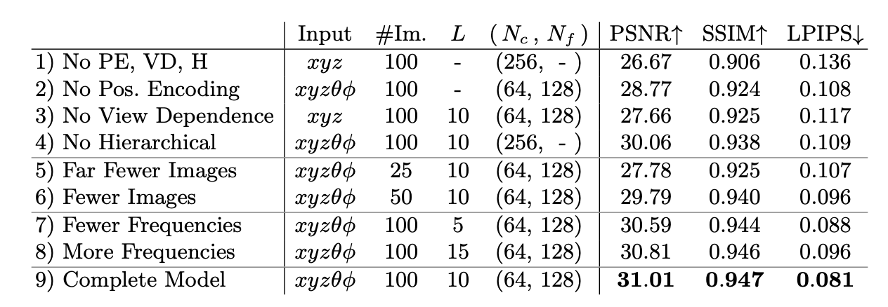
6.4 Ablation studies

7. Conclusion

• 5D neural radiance fields produce better renderings than previous discretized voxel representations
• Still much more pregress to be made in efficiency of both optimizing and rendering
• Interpretability as also future work.