[Paper Review] YOLO: You Only Look Once

지윤·2025년 10월 26일

You Only Look Once:Unified, Real-Time Object Detection
YOLO (You Only Look Once) revolutionizes object detection by reframing it as a single regression problem. YOLO directly predicts bounding boxes and class probabilities from full images with just one network evaluation. This unified approach enables real-time performance (up to 45 fps), simple pipeline, and strong generalization across domains. While YOLO is extremely fast and reduces background errors, it may struggle with small or clustered objects due to its grid-based structure. Overall, YOLO stands out as an efficient and practical standard for modern visual recognition tasks.

1. Introduction

The human visual system can process images quickly and accurately, identifying objects and determining their locations and interactions with minimal conscious effort. The goal in computer vision has been to build object detection models that approach this level of performance. Earlier detection models (Deformable Parts Model(DPM) and R-CNN) repurpose classifiers for use as detectors. Classification seeks to identify what an image contains, but object detection goes further by requiring both class and location information.

Therefore, this post will dive deeply into the structural differences between R-CNN/DPM and YOLO. Then I will examine the YOLO model in detail, focusing on its unified architecture, unique loss function.

> Earlier object detection models

- DPM

DPM st <Figure 1: DPM>

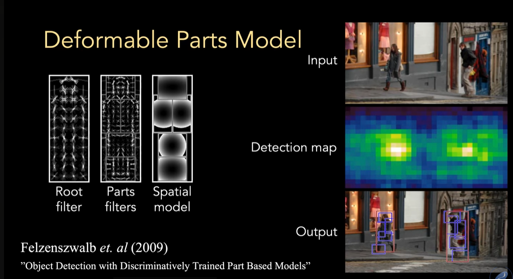
The deformable parts model(DPM) employs filters that correspond to both complete objects and their constituent parts to generate a detection confidence map using a sliding window approach. The underlying idea is that an object is likely present if all of its parts are detected, even when they are arranged in uncommon configurations.

In this model, filters are applied systematically across the image via sliding windows, with each part filter specialized to detect a particular portion of the object. Despite shifts or deformations in the parts’ usual arrangement, the model can still successfully recognize the object, as long as the parts appear within the expected spatial relationships specified by the model’s spatial constraints.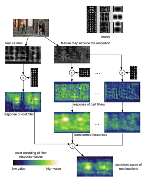 DPM str <Figure 1-2: internal working process of DPM>
As shown in the illustration from Figure 1-2, this pipeline is quite complex. Because it relies on the sliding window approach, the process is slow. Additionally, its detection accuracy tends to lag behind more modern models.

- R-CNN

R-CNN structure <Figure 2: R-CNN>

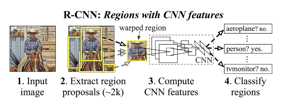
R-CNN generates bounding boxes within an image using a region proposal method. Each proposed bounding box is then classified using a classifier. After classification, bounding boxes are refined, redundant detections are removed, and the scores of the boxes are recalculated based on the object class through a post-processing step. Due to this multi-stage complexity, R-CNN is relatively slow. Additionally, since each step requires separate training, optimizing the entire system is challenging.

R-CNN and its variants (Fast R-CNN, Faster R-CNN) approach object detection by first generating a set of candidate regions in the image called region proposals (ROIs, Regions of Interest). Early models like R-CNN use algorithms such as Selective Search to create up to 2,000 proposals per image. Each proposal is extracted as a sub-image, resized, and sent through a deep neural network for feature extraction and classification, followed by precise boundary box regression.

The original R-CNN pipeline was a series of separate steps: Selective Search generated candidate regions, a convolutional network extracted features, an SVM classified the proposals, a linear model refined the bounding boxes, and Non-Maximum Suppression removed duplicates. Each step was carefully tuned and operated independently, resulting in a slow overall process.
<Figure 2-1: Faster R-CNN Structure>
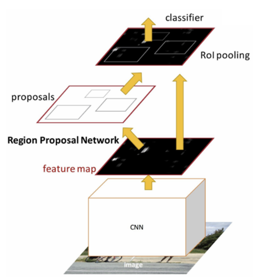
Fast R-CNN improved efficiency by computing a single feature map for the entire image and then using ROI pooling to extract features for all proposals. However, it still depended on external region proposal methods, which caused a bottleneck.

Faster R-CNN integrated a Region Proposal Network (RPN) into the model to generate bounding box candidates directly. While this boosted speed, hundreds of proposals still needed to pass through shared neural network layers for feature extraction, proposal scoring, and classification, limiting real-time performance.

To classify the proposed regions, each must pass through multiple layers of the classifier network. In other words, a CNN (the white box in Figure 2-1) extracts the bounding boxes, and within those bounding boxes, the classifier—which is also a neural network—determines the class of the object.
These are three separate networks with distinct roles, but since they are connected and can be trained end-to-end as a single system, they can be considered as one.

Despite being trained end-to-end, this architecture is fundamentally slow. Real-time speed is slow due to two core issues: the necessary reliance on generating numerous proposals and the unavoidable sequential processing overhead for each proposal through multiple network stages. This design sharply contrasts with YOLO's goal of achieving detection in a single, unified pass.

2. YOLO Architecture

<Figure 3: YOLO Detection System>
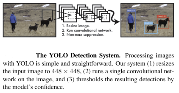
YOLO approaches object detection as a single regression problem, directly mapping image pixels to bounding box coordinates and class probabilities using one unified convolutional network. This simple, end-to-end structure makes YOLO both fast and straightforward, offering clear advantages over earlier, more complex methods

Key Advantages and Features of YOLO

Single Neural Network for Speed and Efficiency
Unlike traditional object detection methods with multiple complex stages, YOLO processes the entire image once, predicting bounding boxes and class probabilities simultaneously, enabling real-time detection.
High Accuracy and Low Background Errors
By considering the entire image context, YOLO better distinguishes objects from background, reducing false positives to less than half compared to some traditional models.
Strong Generalization Ability
YOLO learns generalized object representations, performing robustly even on unseen domains like artwork, outperforming models like DPM or R-CNN.

We can verify the above features through Table 1 of Part 4 Experiment.

2-1. Detection Process

YOLO system <Figure 4-1: YOLO Detection System>
<Figure 4-2>
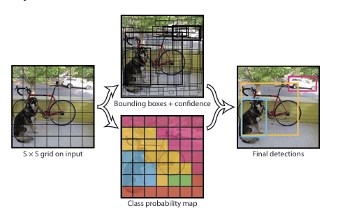
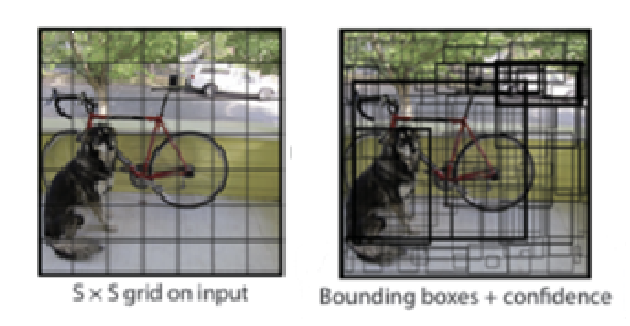
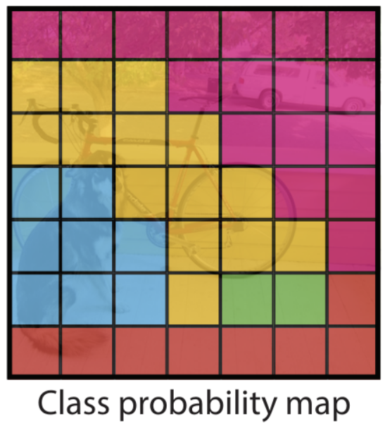
1. Input image is divided into an S×S grid.
2. Each grid cell predicts B bounding boxes and a confidence score for each bounding box. (If no object exists in a cell, its confidence score == zero.)

$confidence score = Pr(Object)×IOUtruth pred$
<Figure 4-3: IoU>
<Figure 4-4>

Each grid cell also contains C conditional class probabilities, $Pr(Class_i|Object)$ .

indicate the probability of each class given that an object exists in the cell.

Each bounding box is represented by x, y, w, h, and a confidence score.

(x, y):represent the center point of the bounding box and are given as values relative to the grid cell's boundaries.
(w, h) indicate the width and height of the bounding box as values relative to the overall image width and height.
Example 1: if x is at the right edge of the grid cell, x = 1; if y is at the top of the grid cell, y = 0.
Example 2: if the bounding box is as wide as the full image, then w = 1.

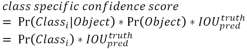
For test, the conditional class probability and bounding box confidence score are multiplied to obtain the class-specific confidence score (These scores encode both the probability of that class appearing in the box and how well the predicted box fits the object.).

Class-Specific Confidence Score = ConditionalClassProbability × ConfidenceScore = <Figure 4-5: class-specific confidence score>

2-2. Network Design

<Figure 5: YOLO network Architecture>
<Figure 5-1: YOLO network Architecture>

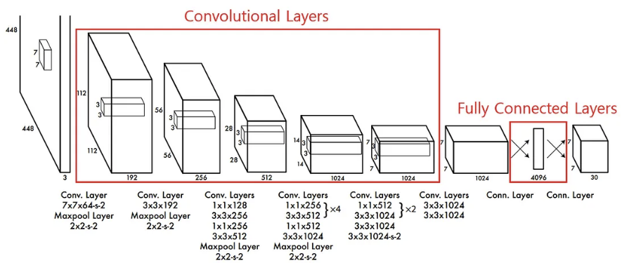
YOLO uses a Convolutional Neural Network (CNN) for object detection, evaluated on the PASCAL VOC dataset. The architecture is inspired by GoogLeNet(Figure 5-2), an image classification model, but differs by replacing GoogLeNet’s Inception block(Figure 5-3). YOLO employs a simpler structure made up of alternating 1x1 reduction layers and 3x3 convolutional layers. The full network consists of 24 convolutional layers followed by 2 fully connected (dense) layers.

For pretraining, the first 20 convolutional layers are trained on the ImageNet classification task with 224x224 images. Then, for object detection, the network accepts 448x448 images as input, and only the final 4 convolutional layers along with the 2 fully connected layers are fine-tuned for detection.

In the forward pass, the convolutional layers extract features from the image, and the fully connected layers predict bounding box coordinates and class probabilities.
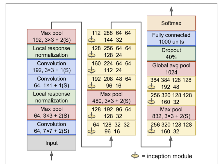<Figure 5-2: GoogLeNet architecture>
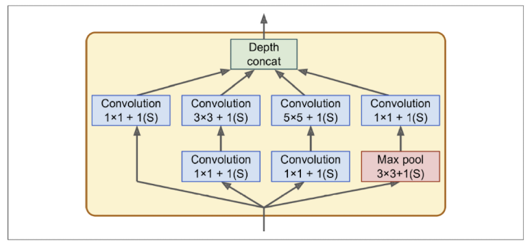<Figure 5-3: Inception module of GoogleNet : YOLO employs a simpler structure made up of alternating 1x1 reduction layers and 3x3 convolutional layers.>

Fast YOLO reduces the number of convolutional layers from 24 to 9 and decreases the number of filters, aiming to improve speed; however, its output structure and training parameters remain the same as the original YOLO.

YOLO's architecture is defined by a straight, unified process that eliminates the complex, multi-stage pipelines of its predecessors:

Image -> CNN -> FC -> PT (Prediction Tensor).

All predictions in YOLO are encoded as a single tensor. The shape of this tensor is S×S×(B×5+C).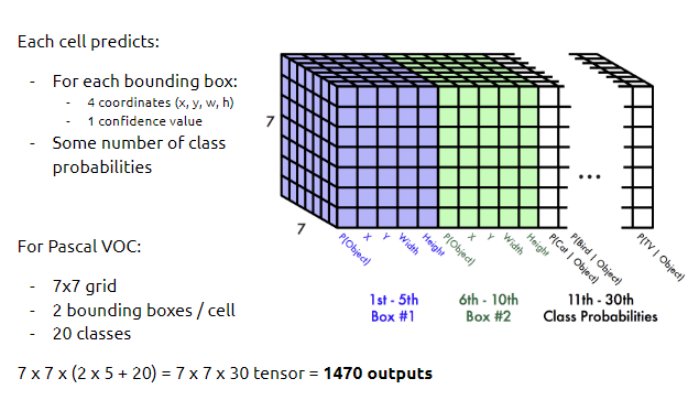<Figure 5-4: visualization of single prediction tensor structure of YOLO>

For the PASCAL VOC dataset, the authors used a grid size of S=7, B=2 bounding boxes per cell, and C=20 object classes.
Plugging in these values gives a final prediction tensor of size: 7×7×(2×5+20)=7×7×30.

2-3. Training

The YOLO model pretrained the first 20 convolutional layers on the ImageNet 1000-class competition dataset. For detection, 4 additional convolutional layers and 2 fully connected layers with randomly initialized weights were added. The final layer predicts class probabilities and bounding box coordinates (x, y, width, height), which are normalized to values between 0 and 1 relative to the image size and grid cell boundaries.
All layers use the Leaky ReLU activation function, except for the final layer, which uses a linear activation function.

YOLO initially opted for Sum-Squared Error (SSE) for optimization due to its ease of use, but it does not perfectly align with the goal of maximizing average precision. SSE presented three key issues:
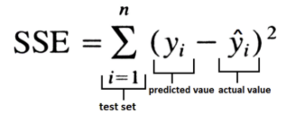<Figure 6: SSE>

SSE is problematic because it weights the localization error and the classification error equally, which is often unsuitable for detection tasks.
Most grid cells in an image do not contain any object. This forces the confidence scores of those empty cells towards 0, creating an instability issue where the massive number of empty cells' gradients overpower the gradients from cells containing objects. This scan cause the model to diverge early in training (make Loss bigger)
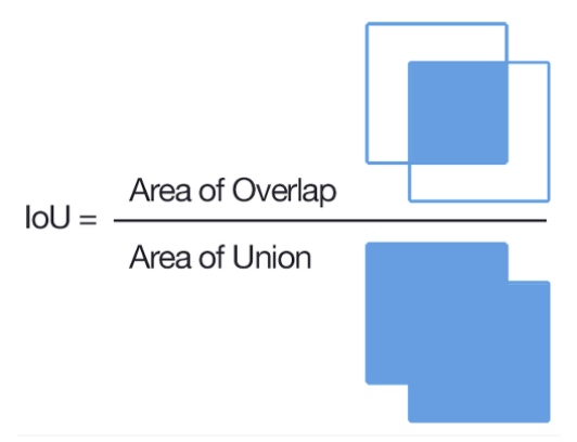
SSE equally weights errors between large boxes and small boxes. Since a small deviation in a small box has a far greater negative effect on accuracy (IOU) than the same deviation in a large box, this equal weighting is inadequate.

To overcome these SSE issues, the loss function was carefully modified:

To address the Instability and Unequal Weighting caused by empty cells, the training introduced two balancing parameters. The loss from bounding box coordinate predictions was increased using $\lambda_{\text{coord}} = 5$ to prioritize accurate box location. Conversely, the loss from confidence predictions in non-object-containing boxes was decreased using $\lambda_{\text{noobj}} = 0.5$ , which prevents the vast number of empty cells from dominating the gradient and ensures stability.
To solve the issue of Unequal Size Weighting, the model was designed to predict the square root of the bounding box width and height ( $\sqrt{w}, \sqrt{h}$ ) instead of the raw values. This change effectively makes the loss function more sensitive to errors in smaller bounding boxes, where precision is most critical for IOU.

This is the multi-part loss function optimized in training:
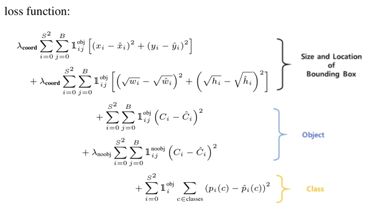<Figure 6-1: Loss Function>

$1_{ij}^{obj}$
: Indicates whether the j-th bounding box predictor in grid cell i is responsible for predicting the object (the one with the highest IOU).
$1_{i}^{obj}$
: Indicates whether an object exists in grid cell i (1 if yes, 0 if not).
$λ_{coord}$
: Balancing parameter that increases the weight for bounding box coordinate loss (x, y, w, h) relative to other terms (typically set to 5).
$λ_{noobj}$
: Balancing parameter that reduces the weight for confidence loss in boxes not containing objects (typically set to 0.5).

Five terms of the loss function, in order, have the following meanings

Bounding box coordinate loss (x, y):
For each responsible predictor (i.e., when $1_{ij}^{obj}$ = 1), compute the sum-squared error between the predicted and ground-truth x, y. These represent the center of the bounding box relative to the grid cell.
Bounding box size loss (w, h):
For each responsible predictor ( $1_{ij}^{obj}$ = 1), compute sum-squared error between the square roots of predicted and ground-truth width and height. The square root reduces sensitivity to large box errors and balances the gradient across large and small objects.
Confidence loss (object present):
For each responsible predictor ( $1_{ij}^{obj}$ = 1), compute sum-squared error between the predicted confidence score and IOU between prediction and ground truth. This penalizes the model when it confidently predicts wrong bounding boxes.
Confidence loss (object absent):
For each bounding box predictor where no object is present (
$1_{ij}^{obj}$ = 0), compute sum-squared error between predicted confidence and 0. This loss is down-weighted by $λ_{noobj}$ , since most boxes in the image will not contain objects.
Conditional class probability loss:
For each cell containing an object ( $1_{i}^{obj}$ = 1), compute sum-squared error for the conditional class probability vector (one-hot for the true class). Note that class probabilities are shared across all bounding boxes for a given grid cell.

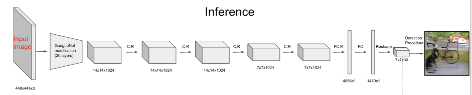
2-4. Inference

The detection prediction process for a single image requires only one inference pass, consistent with the training phase. The grid design of YOLO enhances spatial diversity in predicting bounding boxes. Usually, each grid cell clearly contains an object, so the network predicts one bounding box per object. However, for large objects or those near grid boundaries, Non-Maximum Suppression (NMS) can be applied.
NMS works by removing all bounding boxes associated with the same object except for the one having the highest confidence score. NMS improves mean Average Precision (mAP) by about 2-3% compared to when it is not used.

2-5. Limitation

Since each grid cell predicts only a single class, it struggles to accurately detect multiple small, closely packed objects.
The shape of the bounding boxes is learned solely from the training data, so unusual or new bounding box shapes are not predicted accurately.
Bounding boxes are predicted based on feature maps generated after multiple layers, which can lead to somewhat imprecise localization.

3. Experiments

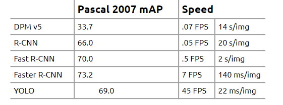<Table 1: Comparison of object detection model accuracy (Pascal 2007 mAP) and speed>
The original R-CNN model achieved high accuracy with 66.0 mAP but required a staggering 20 seconds (0.05 FPS) to process a single image, making real-time deployment impossible. Even its successor, Faster R-CNN, despite further improvements, only reached 7 FPS while achieving a state-of-the-art accuracy of 73.2 mAP, failing to meet the true real-time standard.

YOLO revolutionized this by integrating the inefficient multi-stage architecture into a single regression problem. YOLO maintained a competitive accuracy of 69.0 mAP while dramatically boosting speed to 45 FPS. This speed is over six times faster than Faster R-CNN (7 FPS), with an image processing time of only 22 milliseconds.

This numerical evidence proves that YOLO was the first model to successfully meet the real-time standard while maintaining high accuracy. YOLO demonstrated the efficiency of its single-pass architecture, successfully breaking the speed-accuracy trade-off that previous models failed to overcome.
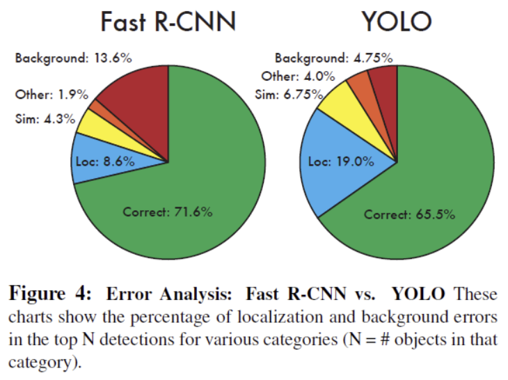<Table 2: VOC 2007 Error Analysis>
YOLO struggles with localization, exhibiting a relatively high localization error rate of 19.0%, which exceeds all other error types combined at 15.5%. However, YOLO's unified approach is advantageous in reducing false alarms; compared to Fast R-CNN, YOLO makes significantly fewer background errors. Conversely, while Fast R-CNN has smaller localization errors, its background error rate is three times larger than YOLO's.

YOLO's high localization error and Fast R-CNN's high background error were complementary weaknesses that led the authors to introduce a combined model in the paper to significantly boost overall detection accuracy.

4. Discussion

YOLO successfully redefined object detection by reframing it as a single regression problem. This unified approach was the key innovation that allowed YOLO to achieve competitive accuracy and speed, essential for the efficiency needed in modern AI applications.

However, analysis of the base YOLO model reveals clear room for improvement:
Localization Error: YOLO suffers from relatively higher localization errors (19.0%), indicating that its single-pass, grid-based approach struggles with precise boundary prediction.
Small Object Challenge: The grid structure inherently limits its ability to detect small or clustered objects effectively.

YOLO's success marked the beginning of the modern era of single-stage detection. Going forward, I am interested in exploring how later versions like YOLOv3 and YOLOv5 have tackled the core challenges of localization accuracy and small object detection, while preserving the original model’s remarkable speed.

References

YOLO CVPR 2016