의사결정나무
- 스무고개 하듯이 예/아니오 질문을 반복하며 학습하는 모델
- 특정 기준(질문)에 따라 데이터를 구분하는 모델
- 분류와 회귀에 모두 사용 가능
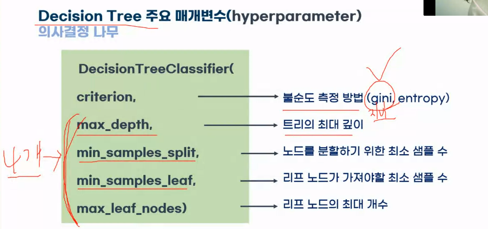
Decision Tree 주요 매개변수(hyperparameter)
- criterion : 불순도 측정 방법(gini, entropy)
- max_depth : 트리의 최대 깊이
- min_samples_split : 노드를 분할하기 위한 최소 샘플 수
- max_samples_leaf : 리프 노드가 가져야할 최소 샘플 수
- max_leaf_nodes : 리프 노드의 최대 개수
Mushroom Dataset을 통해 독성인지, 식용인지 구분
- 8124개의 버섯 종류 데이터
- 22개의 특징(18개의 버섯 특징, 4개의 다른 특징(Habitat(서식지), Population(분포 형태), Bruises(타박상), Odor(냄새))
- 라벨 : 독성(p), 식용(e)
목표
- 버섯의 특징을 활용해 독/식용 이진분류 해보기
- Decision Tree 모델 활용해보기
- Decision Tree 학습현황 시각화 & 과대적합 제어(하이퍼 파라미터 튜닝)
- 특성의 중요도를 파악하기(불순한 정도를 파악하는 것: 지니계수)
1. 라이브러리 호출
import pandas as pd
import numpy as np
import matplotlib.pyplot as plt

from sklearn.model_selection import train_test_split
#train, test 랜덤 샘플링 도구
2. 데이터 불러오기
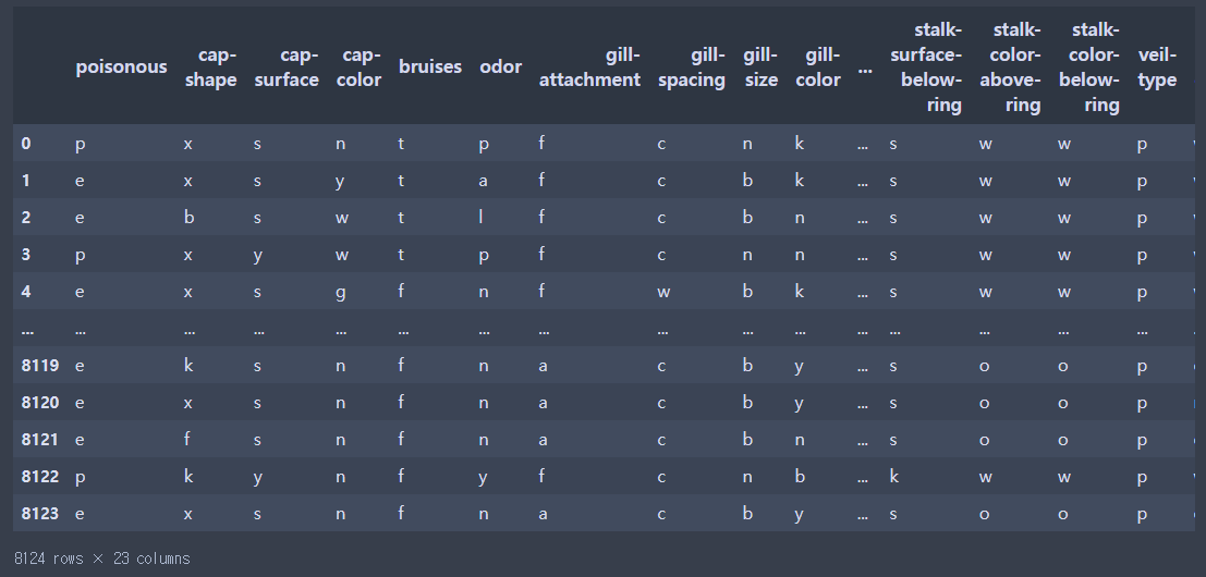
data폴더에 있는 mushroom 가져와서 data변수에 담기
pd.options.display.max_columns = None #모든 컬럼 표시
data = pd.read_csv("mushroom.csv")

data
pd.options.display.max_columns = None : 생략없이 모든 컬럼을 표시한다.
데이터 정보 확인
data.info()

<class 'pandas.core.frame.DataFrame'>
RangeIndex: 8124 entries, 0 to 8123
Data columns (total 23 columns):
#컬럼 인덱스
 #   Column                    Non-Null Count  Dtype
---  ------                    --------------  -----
 0   poisonous                 8124 non-null   object
 1   cap-shape                 8124 non-null   object
 2   cap-surface               8124 non-null   object
 3   cap-color                 8124 non-null   object
 4   bruises                   8124 non-null   object
 5   odor                      8124 non-null   object
 6   gill-attachment           8124 non-null   object
 7   gill-spacing              8124 non-null   object
 8   gill-size                 8124 non-null   object
 9   gill-color                8124 non-null   object
 10  stalk-shape               8124 non-null   object
 11  stalk-root                8124 non-null   object
 12  stalk-surface-above-ring  8124 non-null   object
 13  stalk-surface-below-ring  8124 non-null   object
 14  stalk-color-above-ring    8124 non-null   object
 15  stalk-color-below-ring    8124 non-null   object
 16  veil-type                 8124 non-null   object
 17  veil-color                8124 non-null   object
 18  ring-number               8124 non-null   object
 19  ring-type                 8124 non-null   object
 20  spore-print-color         8124 non-null   object
 21  population                8124 non-null   object
 22  habitat                   8124 non-null   object
dtypes: object(23)
memory usage: 1.4+ MB
info로만 봤을 때는 결측치가 없다는 것을 알 수 있으며 모든 컬럼에는 문자열 데이터만 들어있다.
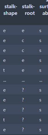
stalk-root : ? 데이터가 들어있다. 이는 지금 바로 건드리는게 아니라 stalk-root데이터를 항상 고려하면서 진행해야하는 것이다.
3. 데이터 전처리 및 탐색
머신러닝은 숫자밖에 학습하지 못한다. 문제(특성)와 답(레이블)을 분리한다.
- X,y 통계량 간단하게 확인
- 머신러닝 모델은 숫자만을 인식한다. 문자 -> 숫자로 변환
- 훈련셋, 테스트셋 분리
버섯의 특징을 활용해 독/식용을 판단하기 위해서 poisonous는 답데이터가 될 것이다. poisonous : y
0 poisonous 8124 non-null object그 외에 컬럼(특성)들은 문제데이터가 될 것이다. 나머지 : X
4. 문제 데이터, 답 데이터 분리
X = data.iloc[:,1:]
y = data.iloc[:,:1]
열 접근
y = data['poisonous']5. 통계량 확인(문제 데이터)
문제 데이터들이 정수라면 평균, 중앙값, std, 최소, 최대등과 같이 분석을 할 수 있을 것이다. 그러나 모든 수가 문자이다.
describe()
X.describe()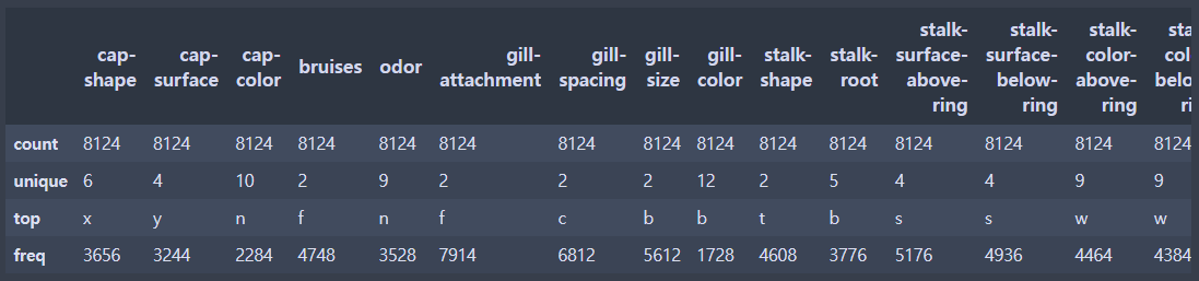
이와같이 문자 데이터(범주 데이터)에 대한 통계는 최빈값, 유니크한 값을 표현해준다.
6. y클래스(카테고리) 확인
- y클래스(카테고리) 개수 확인
- y클래스의 다양성이 유지되는 지 확인(레이블의 균형이 맞는지)
y.value_counts()

#
#e    4208
#p    3916
#Name: poisonous, dtype: int64

#eatable 즉 식용이 더 많다.
7. 데이터 전처리 (문자 > 숫자 : encoding(인코딩))
머신러닝은 숫자만을 인식하기 때문에 인코딩 작업을 통해 수치화하는 프로세스가 필요하다.
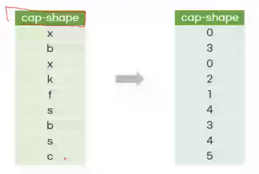
Label Encoding : 레이블을 숫자로 Mapping
X1["capshape"] = X1["capshape"].map({"x":0, "f":1,"k":2....})
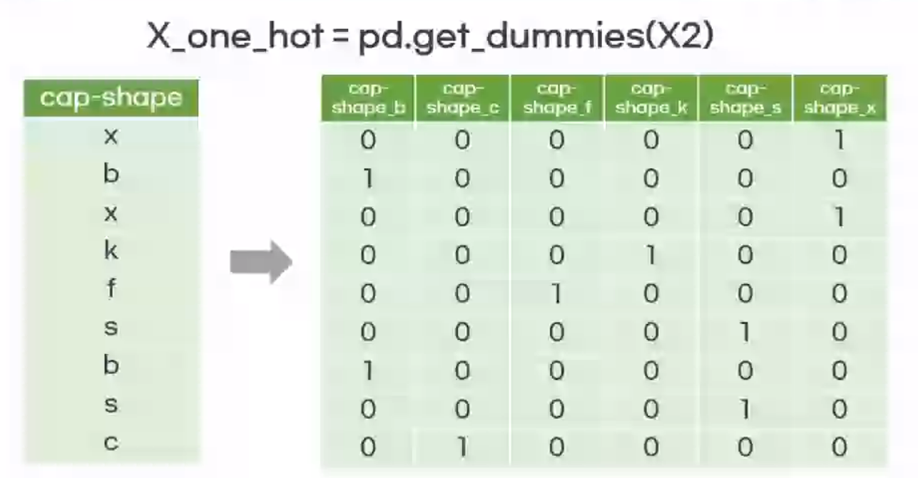
One hot Encoding : 분류하고자 하는 범주(종류)만큼의 자릿수를 만들고 단 한개의 1과 나머지 0으로 채워서 숫자화하는 방식
값의 크고 작음의 의미가 있을 때 : 레이블 인코딩
값의 크고 작음의 의미가 없을 때 : 원 핫 인코딩
따라서 이번 버섯 실습에서는 크고 작음의 의미가 없으므로 원 핫 인코딩을 수행한다.
X_one_hot = pd.get_dummies(인코딩 대상)
X_one_hot = pd.get_dummies(X)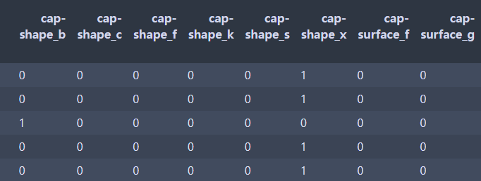
위와 같이 컬럼이 분리돼서 1과 0으로 출력된다.
크기확인
print(X_one_hot.shape)

(8124, 117)
8. 훈련셋, 테스트셋 분리
- 7:3 비율 랜덤스테이트 7
X_train, X_test, y_train, y_test = train_test_split(X_one_hot,y,test_size=0.3, random_state = 7)크기 확인
print(X_train.shape)
#(5686, 22)

print(X_test.shape)
#(2438, 22)

print(y_train.shape)
#(5686,)

print(y_test.shape)
#(2438,)

#훈련데이터, 테스트데이터의 수가 같아야 한다.
9. 모델링
9.1 모델 생성
tree_model 변수에 모델 생성
tree_model = DecisionTreeClassifier()


DecisionTreeClassifier(`shift + tab`누르면 기본적으로 제공하는 것들을 확인할 수 있다.) 기본값으로 설정
9.2 모델 학습
tree_model.fit(X_train,y_train)10. 교차 검증
교차검증 : 모델의 일반화 성능 확인
모든 데이터에 대해 모델이 얼마나 잘 맞추는지 평가하는 것으로 한 번 나눠서 평가하는 것보다 여러 번 하기 때문에 더 안정적인 통계적인 평가 방법이다.
방법론 : 훈련 세트와 테스트 세트로 여러번 나눠서 평가
진행 시점 : 모델을 생성하고 학습하기 전에도 진행 가능
#도구 불러오기
from sklearn.model_selection import cross_val_score

#교차검증
#cross_val_score(estimator,X,y=None,cv=None,)
#문제, 답데이터, cv(cross validation) : 교차 검증 횟수(테스트를 분리할 횟수)

cv_result = cross_val_score(tree_model,X_train,y_train,cv=5)
교차 검증 결과
cv_result
교차검증 평균
cv_result.mean()
5번 진행한 결과 대부분 100%성능을 내고 있어 나름대로 신뢰할만한 모델이라고 판단할 수 있다. 모델의 하이퍼 파라미터를 제어하지 않아도 내부 규칙 생성이 알맞게 됐다. p인지 e인지 판단하기 위한 특성 설명이 충분했다. 하이퍼 파라미터를 제어하지 않아도 되는 상황이다.
11. 모델 예측 및 평가
예측
테스트로 분리한 X_test로 X_train으로 학습시킨 모델을 이용해서 예측하여 실제 데이터와 차이를 확인해보자.
#모델.predict(문제)

pre = tree_model.predict(X_test)
pre

#array(['p', 'p', 'e', ..., 'e', 'e', 'p'], dtype=object)
평가
#도구 호출
from sklearn.metrics import accuracy_score
accuracy_score(y_test,pre)

#1.0 정확하게 출력되었다.
12. 특성 중요도 확인
- 모델 특성 선택 확인하기
- feature importances 확인하기
컬럼에 대한 중요도
fi = tree_model.feature_importances_
fi
컬럼에 대한 중요도이기 때문에 컬럼의 갯수와 같은 수가 출력이 된다.
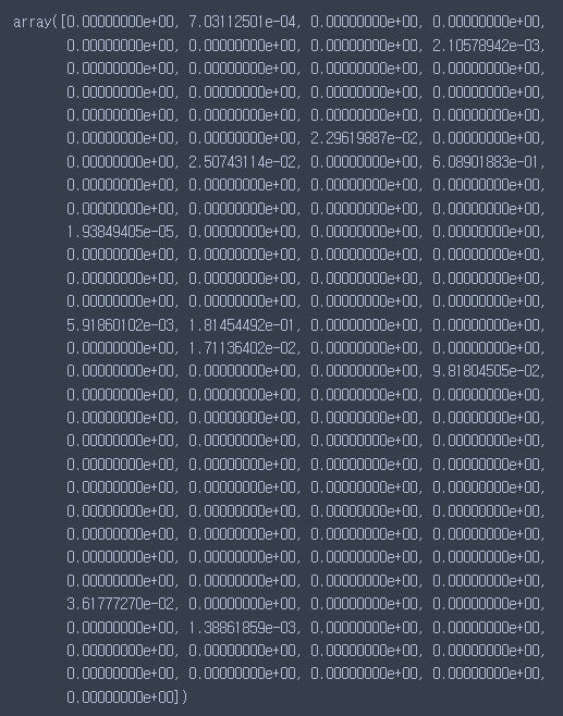
0은 의미가 없다는 것이다.
X_train 컬럼명 출력
X_train.columns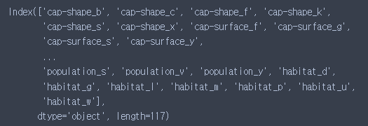
특성 중요도 np배열을 DF로 변환하면서 컬럼명 연결하기
fi_df = pd.DataFrame(fi,index = X_train.columns,columns = ['feature importances'])

fi_df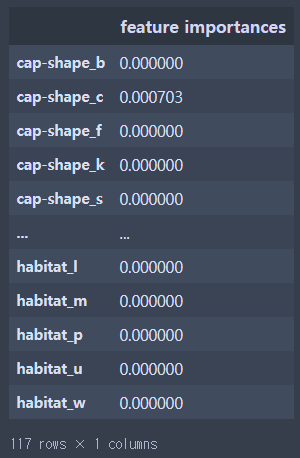
인덱스가 아닌 값을 기준으로 내림차순 정렬
fi_df.sort_values('feature importances',ascending = False)
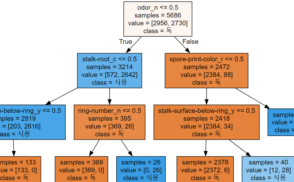
13. 학습 현황 시각화(tree - white box)
그래피즈 다운로드
https://graphviz.org/download/
path 추가

anaconda prompt
pip install graphviz
학습시킨 트리 모델의 현황을 추출하는 코드
from sklearn.tree import export_graphviz
export_graphviz(tree_model, out_file='tree.dot', #추출할 모델
               class_names=['독','식용'], #저장 경로 및 파일명
               feature_names=X_one_hot.columns, #컬럼명
               impurity=False,
               filled=True) #색상을 채우겠다.
위 코드를 실행하면 'tree.dot' 파일이 생긴다.
라이브러리 호출 및 파일 오픈
import graphviz

with open('tree.dot',encoding = 'UTF-8') as f:
    dot_graph = f.read()

dot_graph

display(graphviz.Source(dot_graph))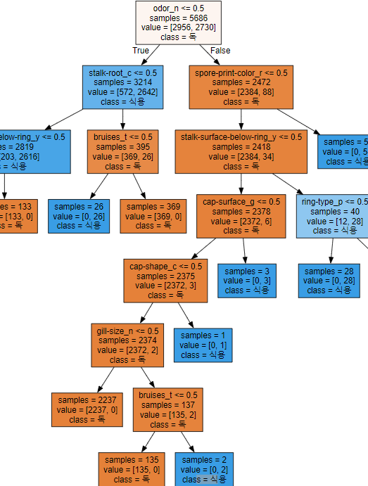
14. 과대적합 제어 후 시각화 확인
tree 모델 하이퍼 파라미터 종류 4가지가 존재한다.
-
max_depth : 트리의 최대 깊이
- 값이 클 수록 모델의 복잡도가 상승한다.
-
max_leaf_nodes : 리프 노드의 최대 개수
- 크게 설정될 수록 분할되는 노드가 증가한다. 개수가 많아진다는 것은 깊이가 깊어진다는 뜻이다.
-
min_samples_split : 노드를 분할하기 위한 최소 샘플 수
- 작게 설정될 수록 분할되는 노드와 복잡드가 상승한다.
-
min_samples_leaf : 리프 노드가 가져야 할 최소 샘플 수
- 작게 설정될 수록 분할되는 도그와 복잡도가 상승한다.
모델의 깊이를 설정하는 매개변수 연결 : max_depth
max_depth를 3까지만으로 설정하고 검증까지 진행해보자.tree_model2 = DecisionTreeClassifier(max_depth = 3) tree_model2.fit(X_train, y_train) train = cross_val_score(tree_model2, X_train,y_train,cv = 5) train #array([0.98242531, 0.98680739, 0.98504837, 0.97977133, 0.98592788]) train.mean() #0.9839960553548712 pre = tree_model2.predict(X_test) pre #array(['p', 'p', 'e', ..., 'e', 'e', 'e'], dtype=object) accuracy_score(y_test,pre) fi = tree_model.feature_importances_ fi_df = pd.DataFrame(fi,index = X_train.columns, columns = ['feature importances']) fi_df.sort_values('feature importances',ascending=False) export_graphviz(tree_model2, out_file='tree.dot', #추출할 모델 class_names=['독','식용'], #저장 경로 및 파일명 feature_names=X_one_hot.columns, #컬럼명 impurity=False, filled=True) #색상을 채우겠다. with open('tree.dot',encoding = 'UTF-8') as f: dot_graph = f.read() dot_graph display(graphviz.Source(dot_graph))```