딥러닝 모델링

모델 구조 설계

딥러닝 모델 도구 불러오기

from tensorflow.keras.models import Sequential

#텐서플로우 라이브러리안에 있는 keras
#Sequential == 모델의 뼈대

from tensorflow.keras.layers import InputLayer, Dense, Activation

#신경망의 구성 요소 (하나씩 조립)'
#InputLayer : 입력
#Dense : 밀집도
#Activation : 활성화함수(인간을 모방하기 위해서 사용하는 함수)

딥러닝 모델 설계 순서

1. 신경망 구조 설계

2. 신경망 학습 및 평가 방법 설정

3. 학습

4. 예측 및 평가

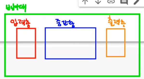
신경망 구조 설계

뼈대 생성 앞으로 모델을 만들거야!

model = Sequential()

입력층 입력 특성의 갯수 작성

model.add(InputLayer(input_shape = (1,))) #studytime

#현재 입력 특성은 studytime 단 한 개이다.

중간층 은닉층이라고도 한다.

model.add(Dense(units = 10))  #뉴런 10개를 연결

활성화 함수 인간을 모방하기 위한 함수(위 선형 함수와 짝꿍)

model.add(Activation('sigmoid')) #활성화함수

출력층 예측할 데이터의 형태

model.add(Dense(units = 1 ))

#성적데이터 1개를 예측하기 위함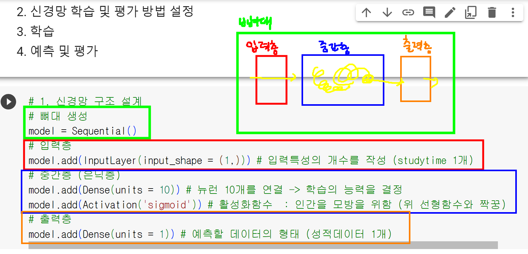

학습 및 평가 방법 설정

딥러닝 모델은 학습법과 평가법을 지정해주어야한다.

model.compile(loss = 'mean_squared_error', optimizer ='SGD', metrics='mse')

#딥러닝 모델을 학습하기 위해서는 LOSS(예측값과 실제값의 차이)값과 최적화 방법(SGD = 확률적 경사하강법), 평가방법을 작성해야 한다.

#loss : 'mean_squared_error' #모델의 잘못된 정도(오차) 측정 알고리즘
#optimizer : 'SGD' #모델의 w,b 값을 최적화하는 알고리즘
#metrics = ['mse']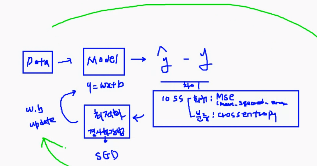

모델 학습

h1 = model.fit(X_train,y_train,validation_split=0.2,epochs =20)

#validation_split : 교차검증을 위한 데이터 남겨두기
#epochs : 모델의 최적화(업데이트 횟수, 반복횟수)
#h1변수에 담는 이유 : 로그를 출력하여 패턴을 확인하기 위함

모델 평가

model.evaluate(X_test,y_test)

#3/3 [==============================] - 0s 5ms/step - loss: 23.8292 - mse: 23.8292
#[23.829193115234375, 23.829193115234375]

모델 학습 로그 출력

h1.history


#{'loss': [96.83131408691406,
#  37.50218963623047,
#  22.583290100097656,
#  19.881580352783203,
#  19.549678802490234,
#  19.439077377319336,
#  19.41645050048828,
#  19.438608169555664,
#  19.394386291503906,
# .....

모델학습 시각화

plt.figure(figsize = (10,5))
plt.plot(h1.history['loss'], label = 'train_loss')
plt.plot(h1.history['val_loss'], label = 'val_loss')
plt.legend()# 범례
plt.show()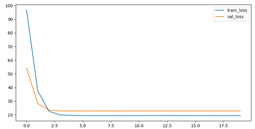

train데이터에 대해서 오차(loss)가 줄어들고 있으며 val데이터도 오차가 줄어든 것을 확인함으로써 일반화 성능이 꽤 괜찮다는 것을 알 수 있다.

---

입력변수를 4개로 설정해보자.

X = data[['studytime','freetime','traveltime','health']]

y = data['G3']

X_train, X_test, y_train, y_test = 
train_test_split(X,y,random_state=918,test_size=0.2)

X_train.shape, y_train.shape, X_test.shape, y_test.shape

model = Sequential()

model.add(InputLayer(input_shape = (4,)))

model.add(Dense(units = 10))

model.add(Activation('sigmoid'))

model.add(Dense(units=1))

model.compile(loss='mean_squared_error',optimizer='SGD',metrics='mse')

h2 = model.fit(X_train,y_train,validation_split=0.2,epochs = 20)

model.evaluate(X_test,y_test)

h2.history

plt.figure(figsize = (10,5))

plt.plot(h2.history['loss'], label = 'train_loss')
plt.plot(h2.history['val_loss'], label = 'val_loss')
plt.legend()# 범례
plt.show()