
🔴Degradation/Restoration
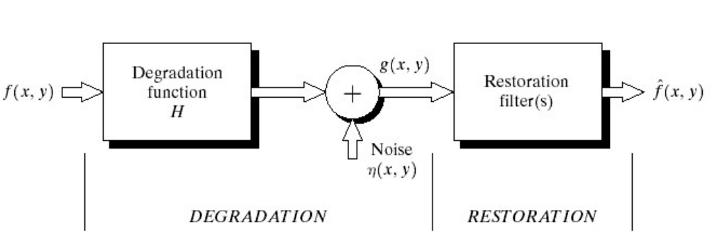
1. Degradation
- 기존의 이미지
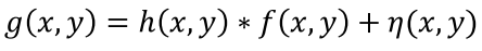
f가 DegradationH을 통해 안좋은 이미지로 바뀐다. 들어간 빛h가 그대로 출력되지 않는 것이다. (ex- 흔들림, 초점, 압축 등) - Noise
η가 더해져 저하된 영상g가 만들어진다.
(뭉개진 사진 + 노이즈)
- Spatial domain
- Frequency domain

2. Restoration
- Degradation된 이미지
g를 복구 - 원본 이미지
f를 모르는 상태로 예상하여 복구하는 것이기 때문에 완벽히 복구는 못한다.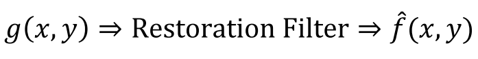
🟠Noise Model
◾ 노이즈의 원인
- Image Acquisition (이미지 획득)
(Sensor에 광자가 쌓이면서 전하도 쌓이는데, 전하를 한꺼번에 뽑아서 한 프레임으로 저장한다. 이 과정에서 깔끔하게 뽑히지 않았거나, 위치 선정이 잘 안되었거나, 튕기게 되면 Noise가 생기게 되는 것이다.)
- Digitization (디지털화)
- Transmission (전송)
➕ White Noise
- Fourier spectrum으로 변환 시, 모든 주파수 영역이 고르게 나타나는 Noise
- Noise를 주파수 영역으로 변환시켰을 때, 스펙트럼이 전부 상수인 경우이다.
- 위치(spatial coordinates), 이미지 자체와 상관 없이 일정하게 노이즈가 발생하는 것이다.
❗아래로 설명되는 Noise들은 확률 밀도 분포(PDF)에 따른 특성을 가진다.
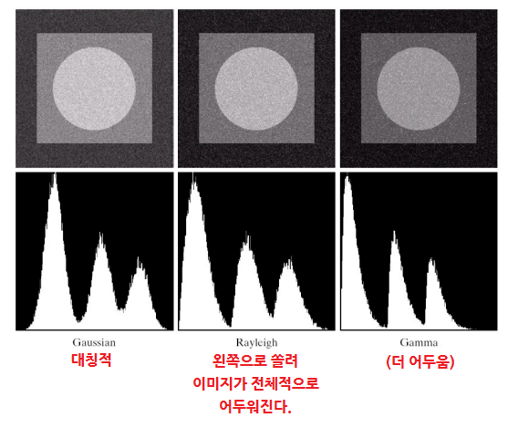
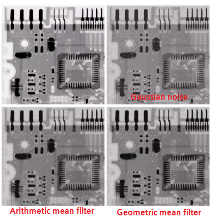
1. Gaussian Noise
- 가우시안 분포를 따르는 Noise
- 평균: μ (z=μ일 때 가장 크다.)
✔️ 어두울 때(Poor illumination) 또는 고온으로 센서에 생기는 Noise. (빛이 적어서 증폭을 늘려주다보니 노이즈가 생김)
✔️ 어두운 환경에서 동작하는 영상 센서에서 발생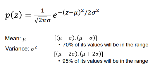
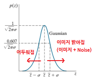
❗중심을 기준으로 오른쪽으로 갈수록 이미지가 밝아지고, 왼쪽으로 갈수록 어두워진다. 다른 노이즈도 마찬가지!
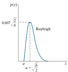
2. Rayleigh Noise
- Rayleigh 분포를 따르는 Noise
- 기우시안에 비해 원점과 가깝고 왼쪽으로 치우쳐져있다.
✔️ 3차원 거리 영상화(range imaging)에서 발생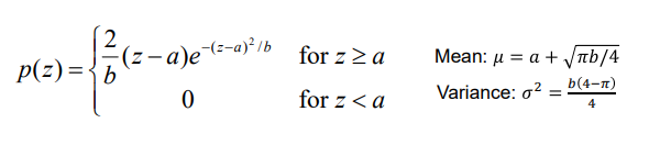
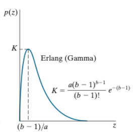
3. Erlang(Gamma) Noise
- a>0, b는 양의 정수인 Erlang 분포
✔️ Laser imaging에서 발생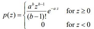
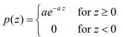
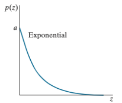
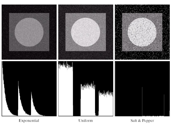
4. Exponential Noise
- a>0인 Exponential 분포
- 아래 그래프를 보면 어두워지는 Noise가 없다.
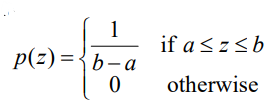
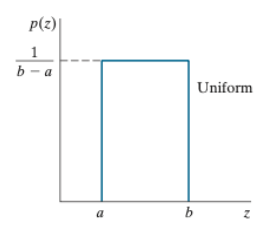
5. Uniform Noise
- z가 없는 Noise이다.
- 고른 분포를 가진다.
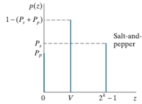
6. Impulse(salt-and-pepper) Noise
- z가 없는 Noise이다.
✔️고장난 스위칭 장치에서 발생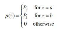
◾Noise PDF의 시각화(Histogram)
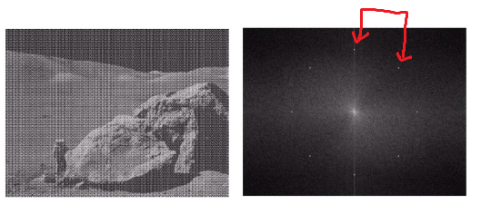
7. Periodic Noise
- 주기를 가지는 Noise.
- DFT를 한 주파수 도메인에서 일정한 패턴을 확인할 수 있다.
◾Noise Parameters 추정
- 주파수 영역 이미지를 분석하여 Noise Parameters를 추정한다.
- 이미지의 특정 부분을 Sampling을 하여 평균과 표준편차 등을 알아내 카메라의 특징을 알아내는 것이다.
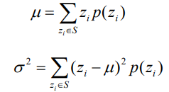
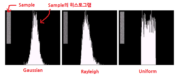
- 이때 평균
μ가 1이 되도록 하는 것이 이미지 복구를 위한 필터링이다.(?)
🟡Restoration in the Presence of Noise Only-Spatial Filtering
✔️Histogram만 보고 원래 식을 알아내기
- 일단 Degradation
H가 없고 Noise만 있는 이미지 복구를 위해 Noise 없애기를 해본다.
(Noise만 있을 때는 DFT를 해도 식이 똑같기 때문)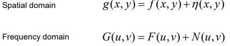
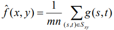
1. Mean Filters
❗산술≥기하≥조화
❗ 평균이 0인 Noise라고 가정
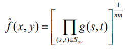
1. Arithmetic meam filter (산술 평균 필터)
- 이전에 등장한 Box filter와 유사하다.
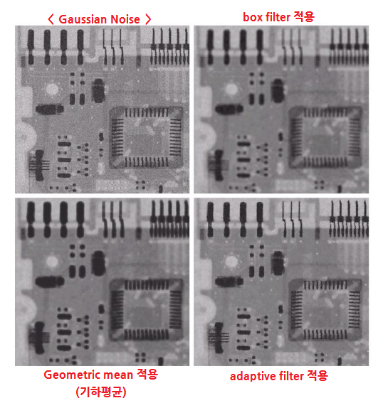
- Gaussian Noise의 경우, 평균이 0인 zero mean이므로 주변과 비교했을 때 평균값이 원본 색임을 알 수 있다. 그래서 이미지의 평균을 구하는 방법으로 Noise를 제거한다.
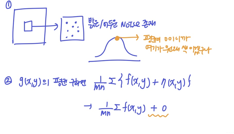
- 산술 평균 필터는 위의 이미지 설명처럼 주로 Noise 평균이 0인 경우에만 사용한다.
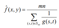
2. Geometric mean filter (기하 평균 필터)
- 산술 평균 필터는 더해서 평균, 기하 평균 필터는 곱해서 평균
(원리는 동일하다.)
- 산술보다 기하가 작기 때문에 기하 평균 필터가 더 어둡다.
3. Harmonic mean filter (조화 평균 필터)
- 역수의 평균을 구한 뒤 역수를 취한다.
- Salt Noise에서는 잘 작동하지만 Pepper Noise는 잘 작동하지 않는다. (큰/밝은 outlier는 크게 영향을 주지 않는다.)
⭐ Outlier와 연관성
- 산술 평균 필터는 outlier에 큰 상관 없지만, 기하와 조화 평균 필터는 outlier에 큰 영향을 받는다.
- 그래서 기하와 조화 평균 필터는 Pepper Noise에 적용하면 안된다.
(어두운 밝기는 0이므로 곱하기 연산 / 역수(분모)에 들어가는 것이 적합히자 않음)
4. Contraharmonic mean filter (콘트라 조화 평균 필터)
- Pepper Noise에서 작동하지 않는 조화 평균 필터의 단점을 보완
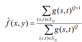
- Q=0 -> 산술 평균 필터
- Q=-1 -> 조화 평균 필터
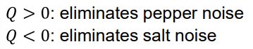
- Q가 커질수록 f값이 Sample의 Maximum쪽으로, 작아질수록 Sample의 Minimum쪽으로 나타난다.⭐
(사실 가늘고 굵어지는 문제가 발생하기 때문에 mean filter만 많이 쓴다..)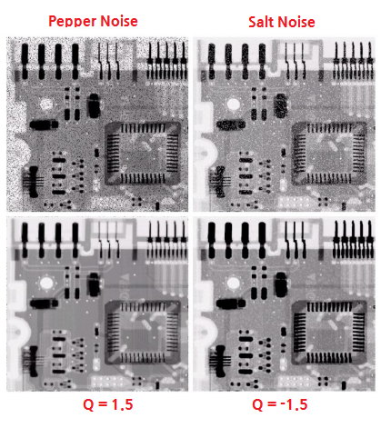
- 만약 Q를 반대로 적용한다면 아래 이미지처럼 된다.
- PepperNoise에 Q가 음수면, Minimum쪽으로 가면서 밝아야될 부분도 어두워지고, SaltNoise에 Q가 양수면, Maximum쪽으로 가면서 어두워야할 부분도 밝아지는 것이다.
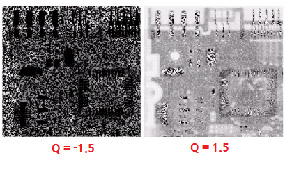
- 결국 Q를 적절히 사용해야하며, 사용자가 고려해야되는 부분이 발생한다.
2. Order-Static Filter
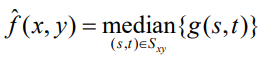
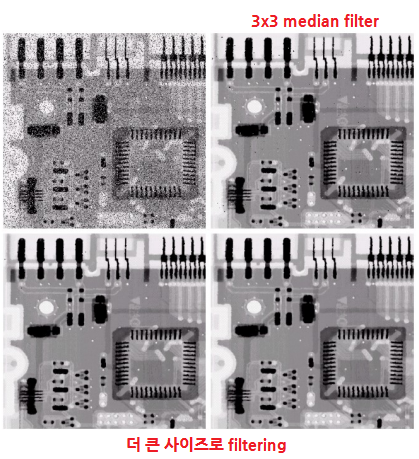
1. Median Filter (중앙값 필터)
- Outlier의 영향을 줄여준다.
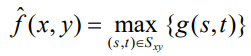
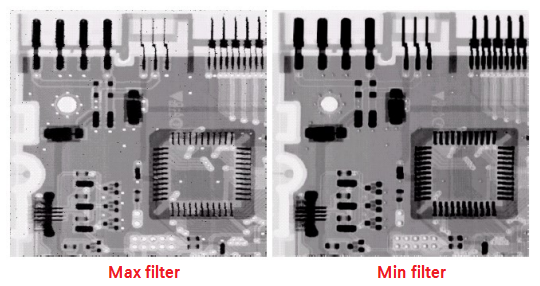
2. Max Filter (최댓값 필터)
- Pepper noise를 줄여준다.(아주 작은/어두운 값의 영향을 없앤다)
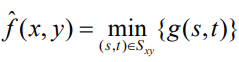
3. Min Filter (최솟값 필터)
- Salt noise를 줄여준다.(아주 큰/밝은 값의 영향을 없앤다)
- 하지만 Max/Min은 가늘고 굵어지는 등의 문제가 발생한다.
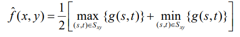
4. Mid-point Filter (중간점 필터) △
- Max와 Min의 평균
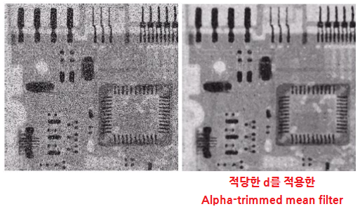
5. Alpha-trimmed mean Filter (알파 트리밍 평균 필터)
- Outlier의 가능성이 있는
d/2개의 가장 낮은 밝기 값들과d/2개의 가장 높은 밝기 값들을 무시한다. (d는 정도를 조절할 파라미터) - 무시한 이미지
gr의 합을 전체 픽셀 수에서 무시한 픽셀 수를 뺀mn-d로 나눈다.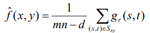
- 하지만 이미지 크기가 작으면 무시할 픽셀이 별로 없다..
❗평균을 바탕으로한 필터의 문제점
- 필터링을 했을 때 뿌옇게 된다(블러).
- 이를 방지하기 위해서 원래 High frequency(Edge)는 살리고 Noise만 삭제해야한다.
- 그래서 Noise의 분포(산포도)를 파악하여, 튀는 픽셀이 Noise인지 edge인지 파악한다. (Adaptive Filter)
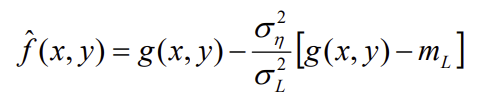
6. Adaptive(Local Noise Reduction) Filter (적응(지역적 노이즈 감소) 필터)
- 영상 내의 통계적 특성에 따라 필터가 변화한다.
- Noise의 분포보다 밖에 있는 튀는 픽셀은 Noise가 아닌 edge일 가능성이 크니까 살리고,
- Noise의 분포 안으로 들어오는 픽셀은 Noise일 가능성이 크니까 무시한다.
- :
g이미지의 전체 산포도 (모델링하여 미리 알고있다.) - : 특정 한 픽셀 주변의 지역적 산포도
- 위 식을 아래와 같이 정리하면 의 비율로
g와m을 섞는 것임을 알 수 있다.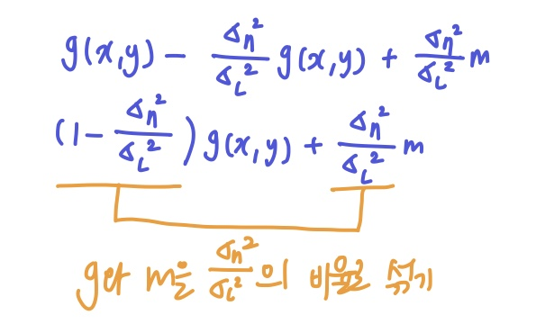
◾ 로 둘 때
- :
g(x, y)만 사용- :
g(x, y)와 가까운 값 ()- :
m만 사용(산술평균)
- 블러되지 않고 / 두꺼워지지도 않게 Noise만 삭제됨
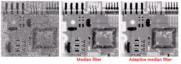
6. Adaptive Median Filter (적응 중앙값 필터)
- 기존 중앙값 필터링에서 하지 못했던 디테일 보존 가능
- Salt-Pepper Noise 제거 / 이외의 다른 Noise는 스무딩 / 얇고 두꺼워지는 현상 보완
- 는 서브 윈도우(박스, 주변 픽셀)을 의미한다.
(zmin은 주변 픽셀 중 가장 작은 값이라고 이해하면 됨)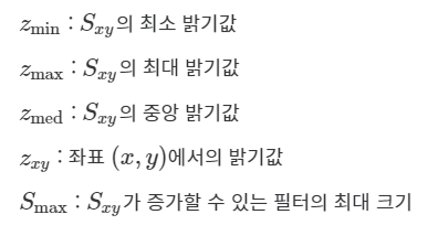
◾Algorithm
- 단계 A는 salt-pepper Noise를 최대한 제거하는 것이기 때문에 단계 B에 해당하는 윈도우 내에서는 salt-pepper Noise가 존재할 가능성이 낮다. 그래서 B에서는 자기 자신이 노이즈인지 확인한다.
- salt-pepper Noise(Outlier)인지 아닌지 파악하는 과정이며 Outlier가 아니면 그대로 사용하고, Outlier라면 Median filter를 적용하는 것이다.
- A단계에서 window size를 늘릴 때, Smax값이 작다면, 정확히 Outlier를 판별할 수 없다.
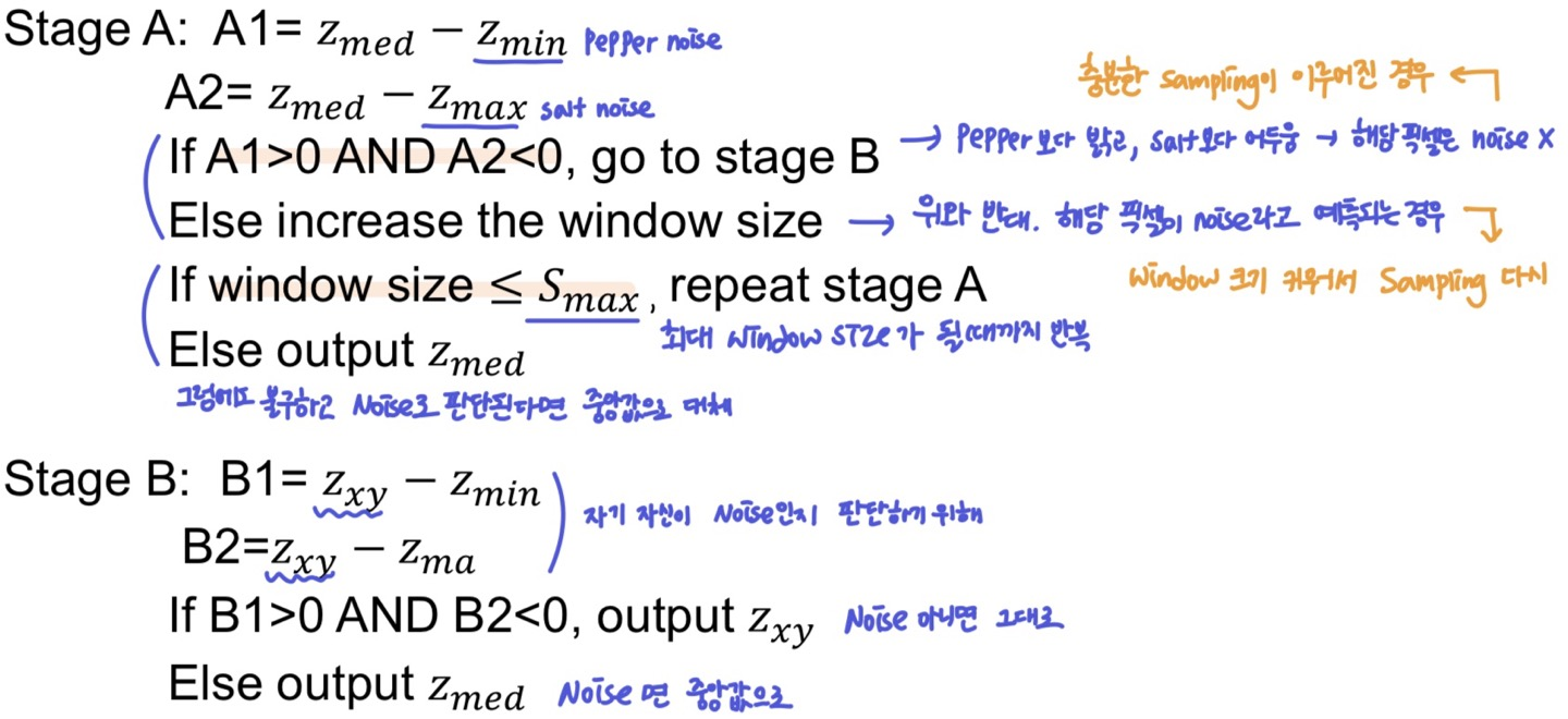
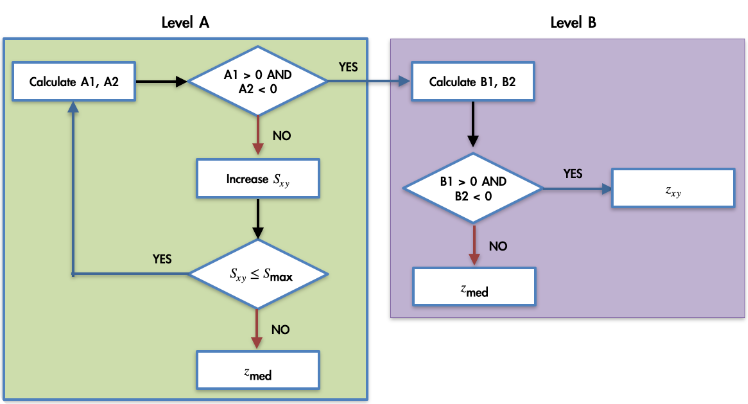
⭐ 시간이 오래 걸린다는 단점이 있다. (확실히 outlier가 아닐 때만 작동하도록 설계되어있으며, 그것을 확인하기 위해 계속 window size를 증가시켜야한다. - iterative(반복적))
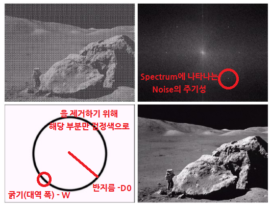
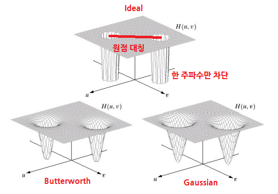
🟢Periodic Noise Reduction
- 주기성을 가지는 Noise는 Frquency domain에 point로 나타나고, 이 그 point의 주파수 성분을 없애기 위해 원 형태(band) 또는 점(notch) 형태로 필터를 만든다.
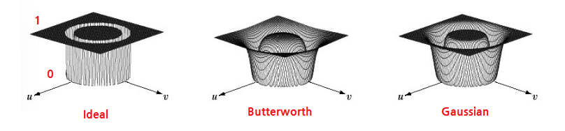
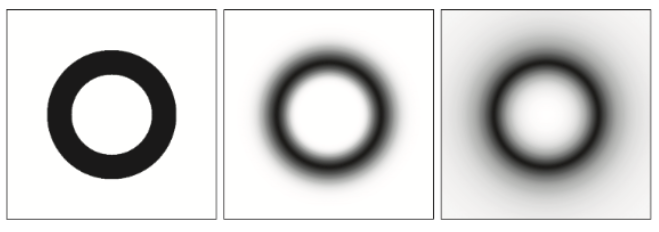
1. Bandreject filters (대역차단 필터)
- 특정 주파수 영역을 차단하는 필터링
1. Ideal bandreject filter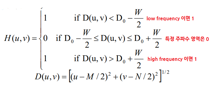
2. Butterworth bandreject filter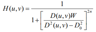
3. Gaussian bandreject filter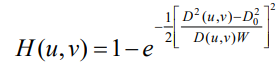
2. Bandrepass filters (대역통과 필터)
- 특정 주파수 영역만 통과시키는 필터링
- 위의 예시로 적용하면 Noise만 보이게 된다.
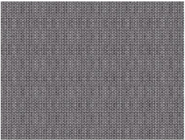
3. Notch filters
- 한 주파수 성분만 차단하는 필터링
- 위의 BP필터처럼 영역을 제거하는 것이 아닌, 특정 점(픽셀)만 제거하는 필터링
- DFT는 대칭구조(원점대칭)를 가지므로 특정 위치, 즉 노치 지점는 반드시 원점에 대칭인 에 대해서 대응 노치를 가진다.
😬 식은 그냥,, 보기만 하기
1. Ideal Notch filter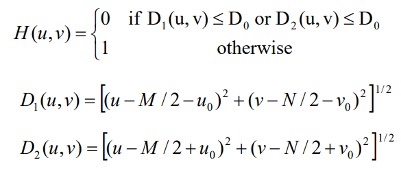
2. Butterworth Notch filter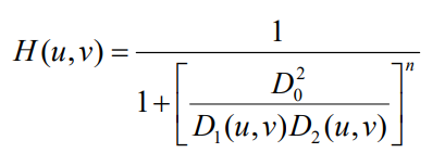
3. Gaussian Notch filter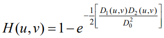
4. Notch pass filter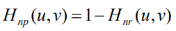
🔵Linear, Position-Invariant Degradations
- 지금까지 Noise가 있는 경우만 생각했다면, 이번에는 Degradation
H가 적용된 경우를 생각한다. - Noise가 없다고 생각할 때
η=0, Input이미지f와 Output이미지g의 관계는 아래와 같다.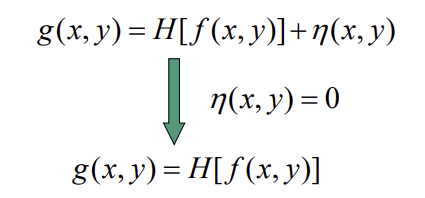
✔️ Property (PSF에 필요한 조건들)
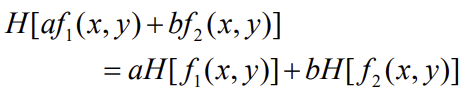
1. Linearity (선형적)
- Additivity, Homogeneity 두 조건을 만족할 때 Linearity하다.
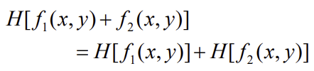
- Additivity (가산성)
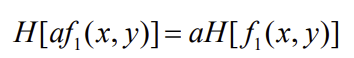
- Homogeneity (동차성)
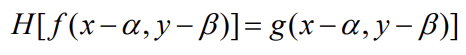
2. Position(or space) Invariant (위치/공간 불변성)
- α, β만큼 평행이동한 다른 위치에 Degradation하면 결과도 평행이동한 위치로 나타난다.
- 위치에 따라 하는 일이 바뀌지 않음을 나타낸다. (
H가 위치에 따라 바뀌지 않는다.)
- Continuous impulse funtion
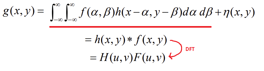
f의 수식에H를 적용하여g를 만들 때 Linear하다면 아래와 같이 유도할 수 있다.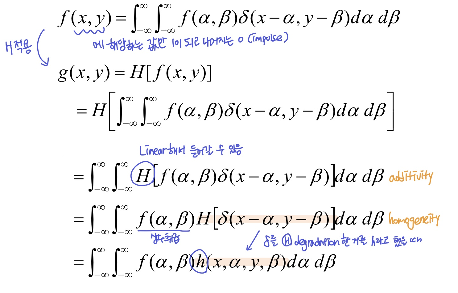
1. Point Spread Funtion
- Point Spread Funtion(PSF)
h는H의 Impulse response이다.
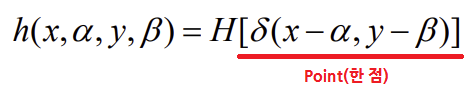
- 광학적으로는, Impulse는 빛의 점을 의미한다.
- 모든 물리적 광학 시스템에서 빛의 점은 어느 정도 번진다(blur/spread).
- 따라서~, Degration Funtion
H가 Linear하고 Position Invariant하면 PSF로 모델링이 가능하다. ⭐
-> 아래 그림처럼 Point를 (Linear하고 Position Invariant한H로)Degradation했을 때, Spread되고 Blur처럼 나타난다.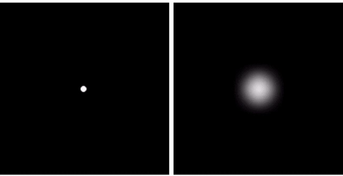
- 모델링한 식은 Convolution형태를 띈다.
➕ Noise가 있는 경우!
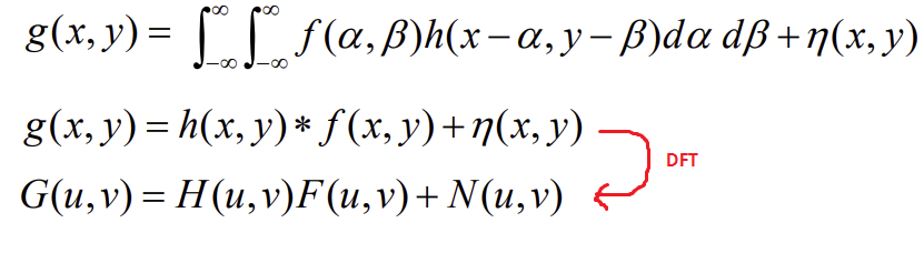
- 따라서, Linear하고 Position Invariant한 Degradation Funtion일 때, PSF를 Convolution한 형태로 만들 수 있다.
❗이미지를 복원(Restoration)하는 것은 Deconvolution하는 것이다!!! (Convolution되있는 상태를 원래대로 돌리기)
🟣Estimating the Degradation Function
- Deconvolution해서 Degradation Function
H를 알아내는 것이 목표 - 어떠한 이유로 손상된 이미지의
H를 알아내면, 원본이미지를 손상된 이미지와 동일하게 직접 만들 수 있게된다. - PSF조건을 만족하는
H가 되는 예시 4가지는 아래와 같다.
1. 영상 관찰
- 노이즈를 뺀 식을 아래와 같이 나타낼 수 있다.
F는 원본이미지로 미리 알고있으므로,G를 측정하면H를 얻을 수 있다.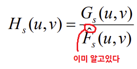
- Spread된 point를 Spread되기 전 원본 point로 만들면 가 상수
A가 된다.(impulse)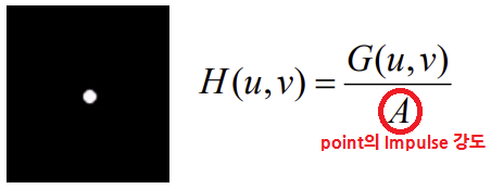
2. 수학적 모델링
(PSF의 조건을 만족하는 예시 3가지)
1. Atmospheric Turbulence (대기의 난기류)
- 빛이 대기 중 영향을 받아 흐트러지는 현상 -> 때문에 뿌옇게 나올 수 있다.
- 난기류를 측정하여 뿌옇게 만드는 것의 수학적 모델은 아래와 같다. (가우시안과 비슷한 형태)
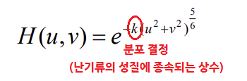
k가 작아질 수록 선명해짐.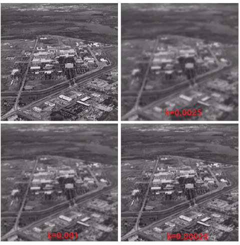
❗두번째 이미지의 k를 알아내서 원본 이미지를 만드는 것이 목표이다.
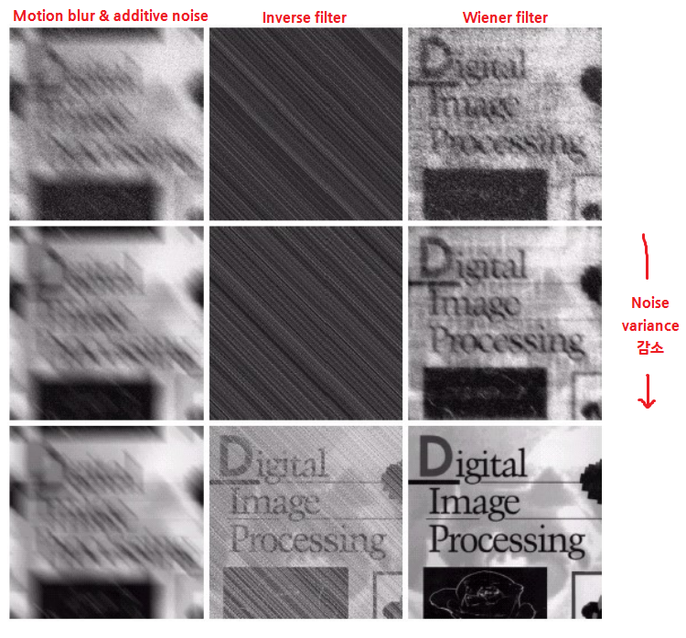
2. Motion Blur (카메라의 흔들림)
- 카메라가 흔들려서 이미지가 뿌옇게 나온 경우
- 시간에 따라 나타낸 x, y방향에서의 움직임 함수
x(t),y(t) - 셔터가 열려있는 아주 짧은 시간
dt동안의 노출들을 적분하여 전체 노출 시간을 얻을 수 있다. - 오염된 영상
g는 아래와 같아지고 정리하면 친숙한 형태의 수식 가 나타난다.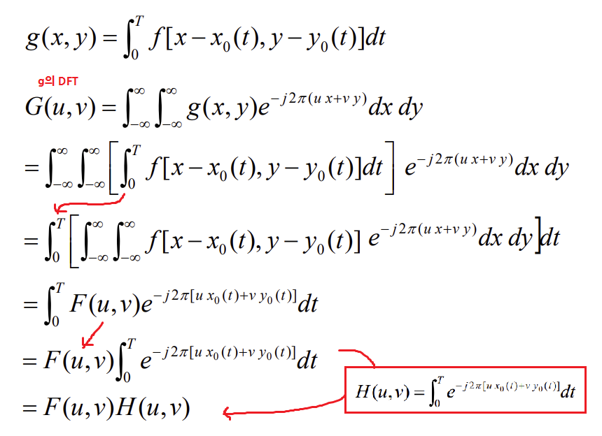
- 따라서, Motion Blur도 PSF이기 때문에 DFT가 가능하고, 이때
h를 DFT한 값이 아래와 같은 것이다. (위의 빨간 박스)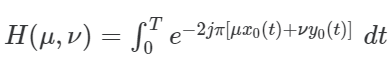
- 만약 사진찍을 때
x쪽으로만 움직인 경우 아래와 같은 식을 만들 수 있는 것이다.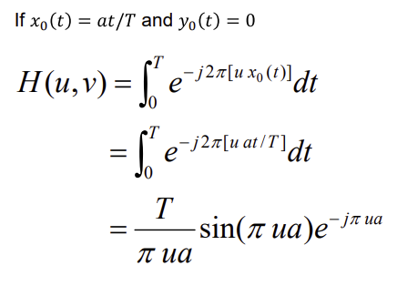
x,y양쪽으로 움직이는 경우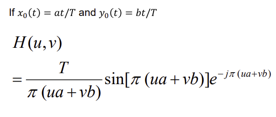
✔️ 위의 식 H를 적용하면 흔들린 사진이 되는 것이다!!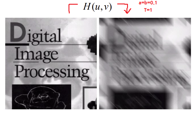
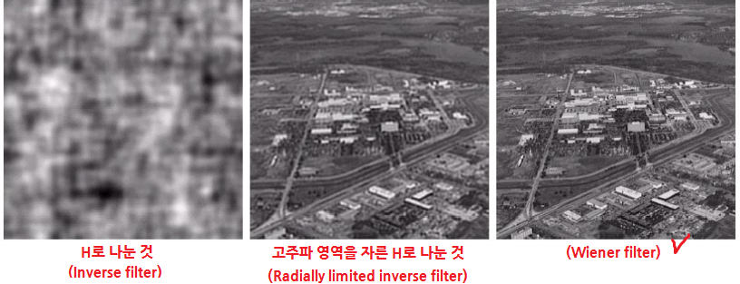
🟤 Inverse Filtering
H를 알아내서 어떻게 이미지가 손상됐는지 알아냈으니까, 이제 거꾸로해서 원본 이미지를 얻어보자- Convolution은 주파수 영역에서 곱셈이니까 Inverse Filtering으로 degradation을 없애려면 주파수 영역에서 나누기를 하면 된다!
- 를 변형해서 아래와 같이 를 알아내는 것이다.
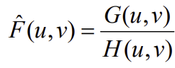
- 식을 계산하면 아래와 같다.
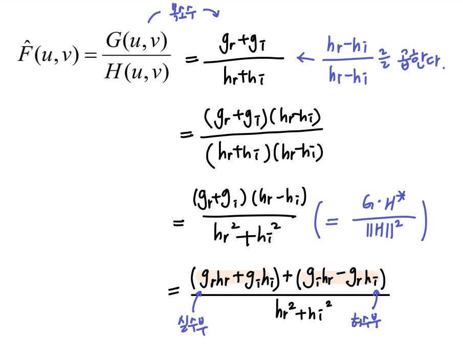
- 하지만 손상된 이미지
G를H로 나누었을 때 원본 이미지F가 나타나지 않는데 이것은 Noise를 고려하지 않았기 때문이다.
(임의로 만든G라도 Noise가 아예 없을 순 없으며, 아주 작은 소수점도 영향을 미치기 때문)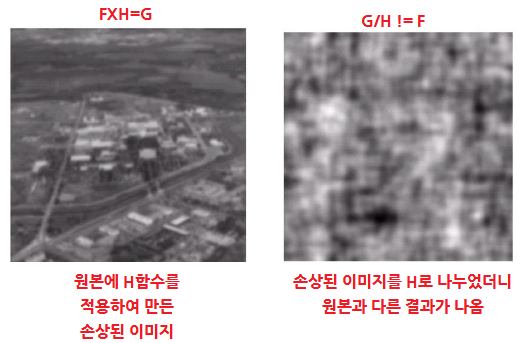
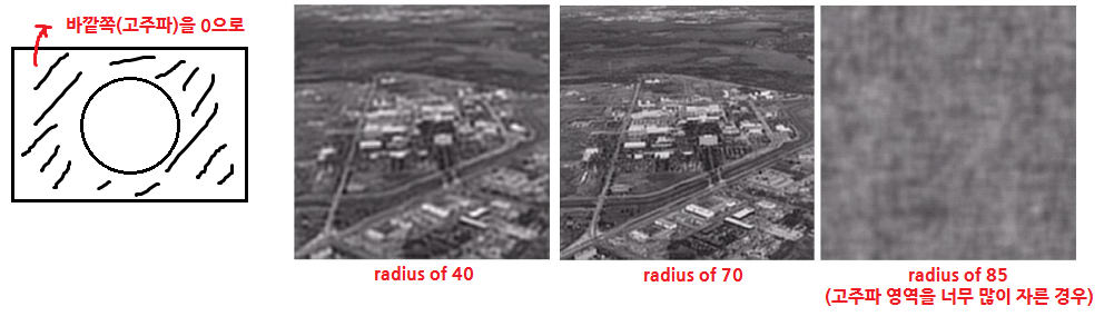
- 그래서 아래 그림과 같이 고주파 성분인 바깥쪽을 잘라내서(0으로 만들어서) 위와 같은 오류가 생기지 않도록 한다.
⚫Wiener Filtering (Minimum Mean Square Error Filtering)
- 최소 평균 제곱 오차 필터
- 위에서 오류가 발생한 것은 아주 작은 소수점도 영향을 미치기 때문이며, 이는 분모가 0에 가까운 값으로 나눠진 이유라고도 할 수 있다.
- 그래서 Wiener Filter로 분모가 0에 가까워지지 않도록 한다.
- errer
e가 최소가 되도록 한다. (의 합의 평균)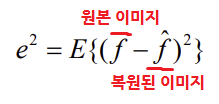
1. Wiener Filter
- 주요 용어
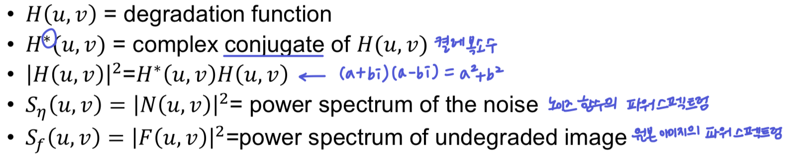
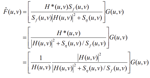
- 위 식에서 를 상수
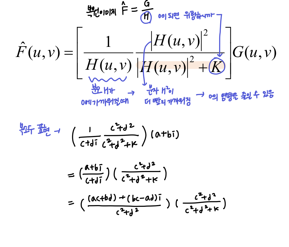
K로 두면 아래와 같다.
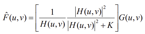
- 위와 같은 식은 분모가 0에 가까워질 때 0의 영향을 줄여준다. 원리는 아래와 같다.
2. Error Measure (SNR/MSE)
- 노이즈의 양을 측정하는 2가지 방법
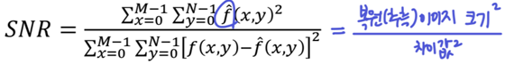
1. MSE (Mean square error)
2. SNR (Signal to Noise Ratio)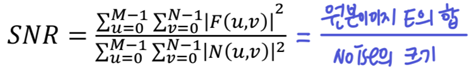
- SNR이 높다는 것은 1. 원본E가 세거나(Signal이 선명) / 2. Noise가 작거나
- SNR이 낮다는 것은 Signal가 약해서 Noise가 도드라진다라고 해석 가능
❗SNR이 높으면 좋다.
- 따라서 복원한 이미지의 SNR은 아래와 같다. (복원 이미지를 신호로, 복원 이미지와 원본 이미지의 차이를 노이즈로 간주한 경우)
( •̀ .̫ •́ )✧