이제는 실제로 구현한 다음 데이터 셋으로 훈련시키고 결과를 확인해 봅시다.

1. 변수 초기화

def __init__(self, learning_rate=0.1, l1=0, l2=0):
    self.w = None              # 가중치
    self.b = None              # 편향
    self.losses = []           # 훈련 손실 기록
    self.val_losses = []       # 검증 손실 기록
    self.w_history = []        # 가중치 변화 기록
    self.lr = learning_rate    # 학습률
    self.l1 = l1               # L1 규제 강도
    self.l2 = l2               # L2 규제 강도

2. 순전파

def forward(self, x):
    # 입력값과 가중치를 행렬곱한 뒤 편향을 더합니다.
    z = np.dot(x, self.w) + self.b
    return z

np는 수치 계산 라이브러리인 numpy를 불러올 때 사용하는 이름입니다. np.dot(x, self.w)는 입력값 $x$와 가중치 $w$의 행렬곱을 계산합니다.

import numpy as np

(np를 사용하기 위해 코드 위에 다음을 추가합니다.)

이 함수는 다음과 같은 선형 연산을 수행하고 그 결과인 $z$를 반환합니다.

반환된 $z$는 이후 시그모이드 함수에 입력됩니다.

3. 역전파

def backward(self, x, err):
    m = len(x)                         # 훈련 데이터 개수
    w_grad = np.dot(x.T, err) / m      # 가중치의 평균 기울기
    b_grad = np.sum(err) / m           # 편향의 평균 기울기
    return w_grad, b_grad

backward()는 오차를 이용하여 가중치와 편향의 기울기를 계산하는 역전파 메서드입니다.

m은 훈련 데이터의 개수이며, x.T는 입력 행렬 x의 행과 열을 바꾼 전치 행렬입니다. err가 $a-y$일 때 기울기는 다음과 같습니다.

계산된 기울기는 이후 가중치와 편향을 수정하는 데 사용됩니다.

4. activation

def activation(self, z):
    z = np.clip(z, -100, None)     # 오버플로 방지를 위해 최솟값 제한
    a = 1 / (1 + np.exp(-z))       # 시그모이드 함수 계산
    return a

5. 모델 훈련

def fit(self, x, y, epochs=100, x_val=None, y_val=None):
    # 실제값을 열 벡터로 변환
    y = y.reshape(-1, 1)

    # 검증 데이터가 있는 경우에만 열 벡터로 변환
    if y_val is not None:
        y_val = y_val.reshape(-1, 1)

    # 훈련 데이터 개수
    m = len(x)

    # 특성 개수에 맞게 가중치 초기화
    self.w = np.ones((x.shape[1], 1))

    # 편향 초기화
    self.b = 0

    # 초기 가중치 저장
    self.w_history.append(self.w.copy())

    # 지정된 횟수만큼 학습 반복
    for _ in range(epochs):
        # 순전파: 선형 출력 계산
        z = self.forward(x)

        # 시그모이드 함수 적용
        a = self.activation(z)

        # 오차 계산
        err = a - y

        # 역전파로 가중치와 편향의 기울기 계산
        w_grad, b_grad = self.backward(x, err)

        # L1·L2 규제 기울기 추가
        w_grad += (
            self.l1 * np.sign(self.w)
            + self.l2 * self.w
        ) / m

        # 학습률을 적용하여 가중치 수정
        self.w -= self.lr * w_grad

        # 학습률을 적용하여 편향 수정
        self.b -= self.lr * b_grad

        # 수정된 가중치 저장
        self.w_history.append(self.w.copy())

        # 수정된 모델로 훈련 데이터 다시 예측
        a = self.activation(self.forward(x))

        # log(0)이 계산되지 않도록 예측값 범위 제한
        a = np.clip(a, 1e-10, 1 - 1e-10)

        # 이진 크로스 엔트로피 손실 계산
        loss = np.sum(
            -(y * np.log(a) + (1 - y) * np.log(1 - a))
        )

        # 규제 손실을 포함한 평균 훈련 손실 저장
        self.losses.append(
            (loss + self.reg_loss()) / m
        )

        # 검증 데이터가 있는 경우에만 검증 손실 계산
        if x_val is not None and y_val is not None:
            self.update_val_loss(x_val, y_val)

fit()은 모델을 학습하는 메서드입니다.

가중치와 편향을 초기화한 뒤, 지정된 횟수만큼 순전파 → 역전파 → 규제 적용 → 가중치 수정 과정을 반복합니다. 수정된 가중치와 훈련 손실을 저장하며, 검증 데이터가 있으면 검증 손실도 함께 계산합니다.

이진 크로스 엔트로피를 계산할 때는 log(0)을 방지하기 위해 np.clip()으로 예측값의 범위를 제한합니다.

6. 값 예측

    def predict(self, x):
        z = self.forward(x)
        return z > 0

시그모이드 함수는 $z=0$일 때 0.5를 출력합니다. 따라서 $z>0$은 시그모이드 출력이 0.5보다 큰 경우와 같습니다.

z > 0의 결과는 True 또는 False이며, 각각 범주 1과 범주 0을 의미합니다.

7. 정확도 계산

    def score(self, x, y):
        return np.mean(self.predict(x) == y.reshape(-1, 1))

score()는 모델의 분류 정확도를 계산하는 메서드입니다.

y.reshape(-1, 1)은 실제값을 예측 결과와 같은 형태의 열 벡터로 변환합니다. 예측값과 실제값을 비교하면 정답은 True, 오답은 False가 됩니다.

np.mean()은 True를 1, False를 0으로 계산하므로 전체 데이터 중 올바르게 분류한 데이터의 비율을 반환합니다.

8. 규제 패널티

    def reg_loss(self):
        return  self.l1 * np.sum(np.abs(self.w)) + self.l2 / 2 * np.sum(self.w**2)

reg_loss()는 L1 규제와 L2 규제에 따른 페널티를 계산하는 메서드입니다. 각 항의 계산식과 역할은 앞서 설명한 L1·L2 규제 식을 참고하면 됩니다.

9. 손실 저장

def update_val_loss(self, x_val, y_val):
    z = self.forward(x_val)                 # 검증 데이터 순전파
    a = self.activation(z)                  # 시그모이드 함수 적용

    # log(0)이 계산되지 않도록 예측값 범위 제한
    a = np.clip(a, 1e-10, 1 - 1e-10)

    # 검증 데이터의 이진 크로스 엔트로피 계산
    val_loss = np.sum(
        -(y_val * np.log(a) + (1 - y_val) * np.log(1 - a))
    )

    # 규제 손실을 포함한 평균 검증 손실 저장
    self.val_losses.append(
        (val_loss + self.reg_loss()) / len(x_val)
    )

update_val_loss()는 현재 모델로 검증 데이터의 손실을 계산하고 val_losses에 저장하는 메서드입니다.

검증 데이터는 가중치와 편향을 수정하는 데 사용하지 않으며, 순전파를 통해 손실만 계산합니다.
저장된 검증 손실은 훈련 손실과 비교하여 과대적합 여부를 확인하는 데 사용됩니다.

모델 학습과 평가

1. 데이터셋 불러오기

사이킷런 패키지에 모델을 학습하고 평가하기 위한 데이터셋을 불러옵니다.

from sklearn.datasets import load_breast_cancer
from sklearn.model_selection import train_test_split
from sklearn.preprocessing import StandardScaler

# 유방암 데이터셋 불러오기
cancer = load_breast_cancer()

x = cancer.data
y = cancer.target

2. 데이터 구분

앞에서 배운 것처럼 불러온 데이터를 훈련데이터, 검증데이터, 테스트 데이터로 나눕니다.

# 전체 데이터를 훈련 80%, 임시 데이터 20%로 분할
x_train, x_temp, y_train, y_temp = train_test_split(
    x,
    y,
    test_size=0.2,
    random_state=42,
    stratify=y
)


# 임시 데이터를 검증 10%, 테스트 10%로 분할
x_val, x_test, y_val, y_test = train_test_split(
    x_temp,
    y_temp,
    test_size=0.5,
    random_state=42,
    stratify=y_temp
)

3. 데이터 표준화

# 특성들의 크기를 맞추기 위한 표준화
scaler = StandardScaler()

# 훈련 데이터로만 평균과 표준편차 계산
x_train = scaler.fit_transform(x_train)

# 검증·테스트 데이터에는 같은 기준 적용
x_val = scaler.transform(x_val)
x_test = scaler.transform(x_test)

4. 모델 학습

model = Singlelayer(
    learning_rate=0.1,
    l1=0.001,
    l2=0.1
)

model.fit(
    x_train,
    y_train,
    epochs=500,
    x_val=x_val,
    y_val=y_val
)

5. 결과 출력

train_error = 1 - model.score(x_train, y_train)
val_error = 1 - model.score(x_val, y_val)
test_error = 1 - model.score(x_test, y_test)

names = ["training", "validation", "test"]
errors = [train_error, val_error, test_error]

plt.figure(figsize=(7, 5))

bars = plt.bar(
    names,
    errors,
    color=["royalblue", "orange", "tomato"]
)

plt.ylabel("error rate")
plt.title("training, validation and test error")
plt.ylim(0, max(errors) + 0.05)
plt.grid(axis="y", alpha=0.3)

# 막대 위에 오류율 표시
for bar, error in zip(bars, errors):
    plt.text(
        bar.get_x() + bar.get_width() / 2,
        bar.get_height(),
        f"{error:.3f}",
        ha="center",
        va="bottom"
    )

plt.tight_layout()
plt.show()

(앞에 import matplotlib.pyplot as plt 입력)

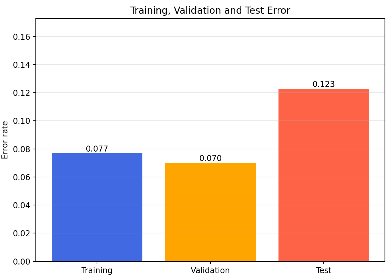
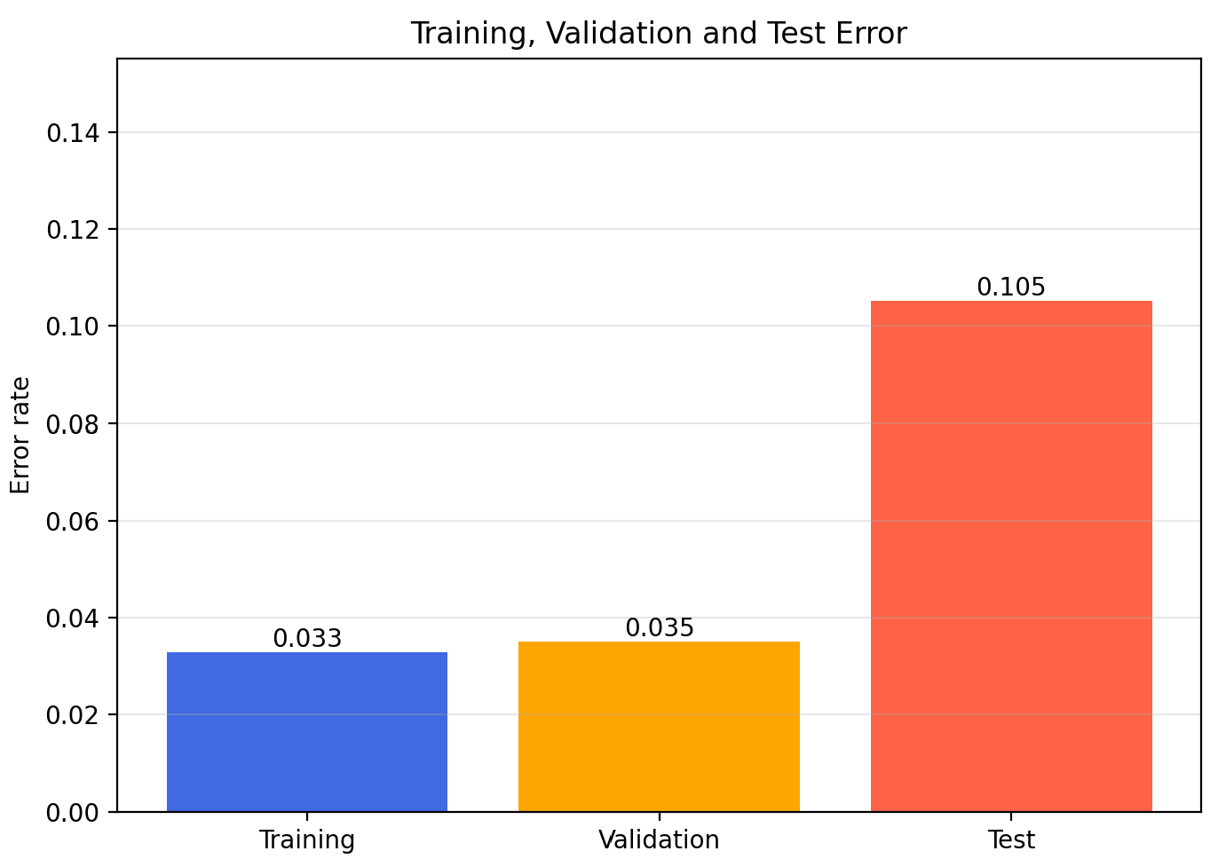
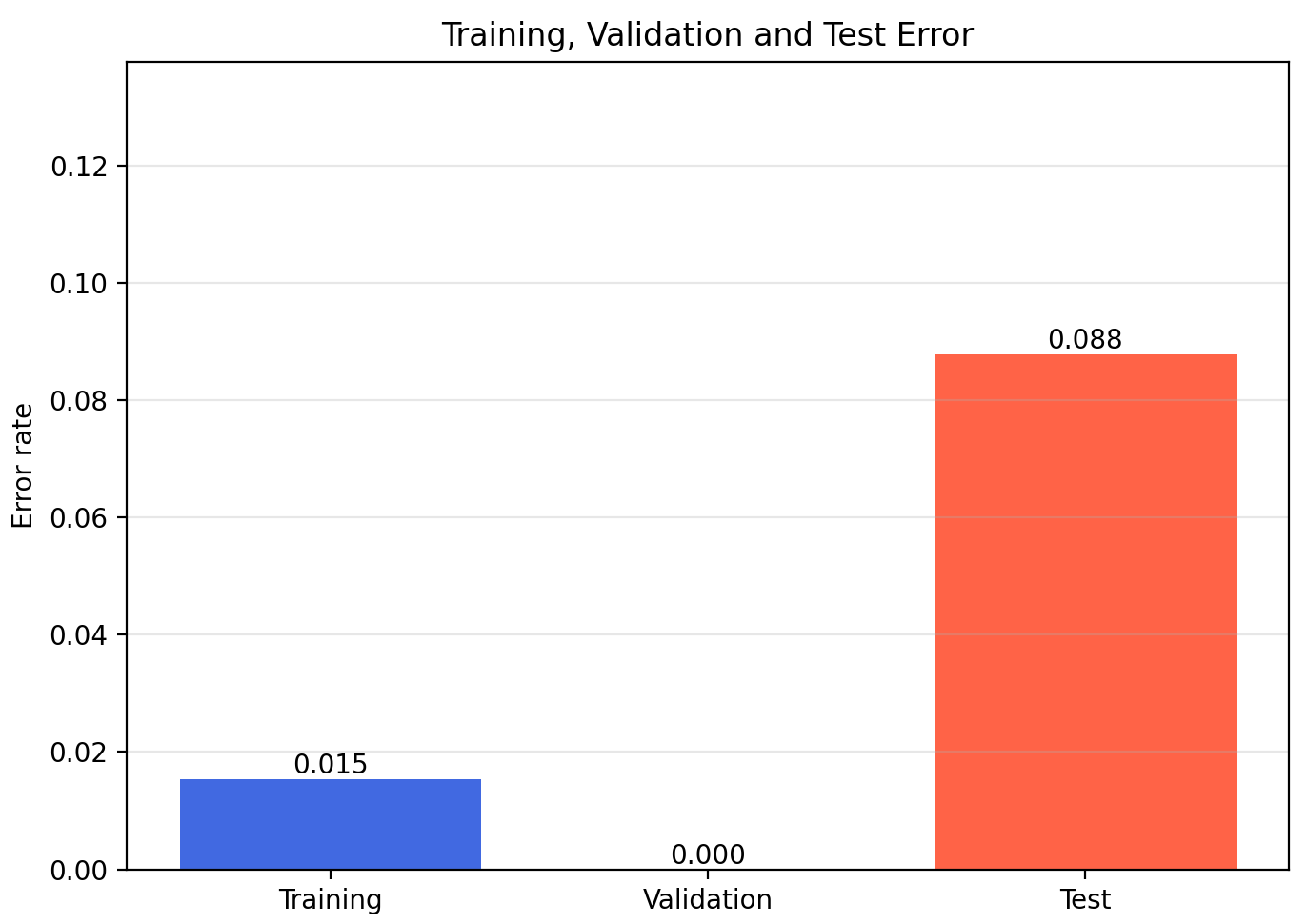
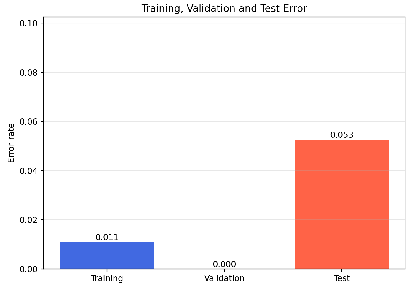
결과

epoch = 50

epoch = 100

epoch = 200

epoch = 500

(전체 코드)

import numpy as np
import matplotlib.pyplot as plt

from sklearn.datasets import load_breast_cancer
from sklearn.model_selection import train_test_split
from sklearn.preprocessing import StandardScaler


class Singlelayer:
    def __init__(self, learning_rate=0.1, l1=0, l2=0):
        self.w = None
        self.b = None
        self.losses = []
        self.val_losses = []
        self.w_history = []
        self.lr = learning_rate
        self.l1 = l1
        self.l2 = l2

    def forward(self, x):
        z = np.dot(x, self.w) + self.b
        return z

    def backward(self, x, err):
        m = len(x)
        w_grad = np.dot(x.T, err) / m
        b_grad = np.sum(err) / m
        return w_grad, b_grad

    def activation(self, z):
        z = np.clip(z, -100, None)
        a = 1 / (1 + np.exp(-z))
        return a

    def fit(self, x, y, epochs=100, x_val=None, y_val=None):
        y = y.reshape(-1, 1)

        if y_val is not None:
            y_val = y_val.reshape(-1, 1)

        m = len(x)

        self.losses = []
        self.val_losses = []
        self.w_history = []

        self.w = np.ones((x.shape[1], 1))
        self.b = 0

        self.w_history.append(self.w.copy())

        for _ in range(epochs):
            z = self.forward(x)
            a = self.activation(z)

            err = a - y

            w_grad, b_grad = self.backward(x, err)

            w_grad += (
                self.l1 * np.sign(self.w)
                + self.l2 * self.w
            ) / m

            self.w -= self.lr * w_grad
            self.b -= self.lr * b_grad

            self.w_history.append(self.w.copy())

            a = self.activation(self.forward(x))
            a = np.clip(a, 1e-10, 1 - 1e-10)

            loss = np.sum(
                -(y * np.log(a) + (1 - y) * np.log(1 - a))
            )

            self.losses.append(
                (loss + self.reg_loss()) / m
            )

            if x_val is not None and y_val is not None:
                self.update_val_loss(x_val, y_val)

    def predict(self, x):
        z = self.forward(x)
        return z > 0

    def score(self, x, y):
        return np.mean(
            self.predict(x) == y.reshape(-1, 1)
        )

    def reg_loss(self):
        l1_loss = self.l1 * np.sum(np.abs(self.w))
        l2_loss = self.l2 / 2 * np.sum(self.w ** 2)
        return l1_loss + l2_loss

    def update_val_loss(self, x_val, y_val):
        z = self.forward(x_val)
        a = self.activation(z)
        a = np.clip(a, 1e-10, 1 - 1e-10)

        val_loss = np.sum(
            -(
                y_val * np.log(a)
                + (1 - y_val) * np.log(1 - a)
            )
        )

        self.val_losses.append(
            (val_loss + self.reg_loss()) / len(x_val)
        )


cancer = load_breast_cancer()

x = cancer.data
y = cancer.target

print("전체 데이터 크기:", x.shape)
print("분류 범주:", cancer.target_names)

x_train, x_temp, y_train, y_temp = train_test_split(
    x,
    y,
    test_size=0.2,
    random_state=42,
    stratify=y
)

x_val, x_test, y_val, y_test = train_test_split(
    x_temp,
    y_temp,
    test_size=0.5,
    random_state=42,
    stratify=y_temp
)

scaler = StandardScaler()

x_train = scaler.fit_transform(x_train)
x_val = scaler.transform(x_val)
x_test = scaler.transform(x_test)

model = Singlelayer(
    learning_rate=0.1,
    l1=0.001,
    l2=0.1
)

model.fit(
    x_train,
    y_train,
    epochs=500,
    x_val=x_val,
    y_val=y_val
)

train_error = 1 - model.score(x_train, y_train)
val_error = 1 - model.score(x_val, y_val)
test_error = 1 - model.score(x_test, y_test)

names = ["training", "validation", "test"]
errors = [train_error, val_error, test_error]

plt.figure(figsize=(7, 5))

bars = plt.bar(
    names,
    errors,
    color=["royalblue", "orange", "tomato"]
)

plt.ylabel("error rate")
plt.title("training, validation and test error")
plt.ylim(0, max(errors) + 0.05)
plt.grid(axis="y", alpha=0.3)

for bar, error in zip(bars, errors):
    plt.text(
        bar.get_x() + bar.get_width() / 2,
        bar.get_height(),
        f"{error:.3f}",
        ha="center",
        va="bottom"
    )

plt.tight_layout()
plt.show()