Anish Acharya, Sujay Sanghavi, Li Jing, Bhargav Bhushanam, Dhruv Choudhary, Michael Rabbat, Inderjit Dhillon
Preprint

1. Introduction

---

머신러닝에서 중요한 주제 중 하나는 라벨이 있는 데이터가 한정된 상황에서 어떻게 하면 효율적으로 학습할 수 있을지를 연구하는 일이다.

기존에는 unlabeled data를 갖고 먼저 self-supervised pretraining을 돌린 후 labeled data를 갖고 supervised fine-tuning을 하는 방법이 주류를 차지하고 있었다. 이때 unlabeled data의 representation을 학습하는 방식으로 널리 사용된 게 contrastive learning이다.

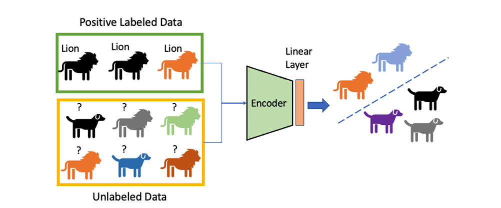
여기서 우리는 contrastive learning을 확장해서 PU(Positive Unlabeled) learning 세팅에서도 이를 활용하고자 한다. PU learning이란, 데이터의 라벨이 positive 혹은 unlabeled만 존재하는 경우를 말한다. 예를 들어, 추천 시스템은 유저가 어떤 컨텐츠를 클릭했는지(다시 말해, 어떤 컨텐츠를 좋아하는지)와 클릭하지 않았는지만 알 뿐, 어떤 컨텐츠를 싫어하는지는 알지 못한다.

따라서 우리의 목표는, weak supervision을 잘 활용해서(즉, unlabeled 데이터에 '암묵적으로' 매겨진 라벨을 활용해서) positive/negative를 잘 구별할 수 있는 적절한 representation $g_B(x)$를 학습하는 것이다.

이를 위해 나온 것이, 이 논문의 핵심인 puNCE(positive unlabeled Noise Contrastive Estimation)이다. puNCE의 메인 아이디어는 다음과 같다:

• unlabeled data는 positive와 negative가 섞인 distribution을 따른다. 이때 섞인 비율은 class prior $\pi$를 따른다.
• puNCE는 각각의 unlabeled sample을 특정 확률에 따라 positive와 negative로 취급하고, 나중에 positive labeled sample의 정보를 활용해서 positive라고 칭해진 샘플들이 같은 embedding space에 모이도록 한다.

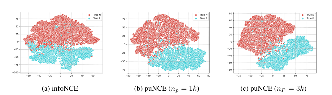
이를 통해 puNCE는 기존 방법인 infoNCE 등을 상당히 개선했다고 한다.

2. Problem Setup

---

2.1. Positive Unlabeled Learning

PU 세팅에서 데이터는 다음과 같은 형태를 따른다:

여기서 $\mathcal{X}_P$는 positive set, $\mathcal{X}_U$는 unlabeled set이다. 이 세팅에서 일단 라벨이 존재하면 무조건 positive이기 때문에, 라벨 존재 여부를 나타내는 변수 $s$를 사용한다. $s=1$이면 해당 샘플은 라벨이 존재한다는 의미이고, 따라서 무조건 positive(즉, $y=1$)이다.

우리는 이제 데이터를 $y$ 없이 $(x,s)$로만 표현할 수 있게 된다.

다음으로 넘어가기 전에 한가지 가정을 세우고 가자.

Assumption 1 (Known Class Prior).
class prior $\pi=p(y=+1)$는 이미 알려져있거나 혹은 mixture proportion estimation algorithm을 활용하여 $\mathcal{X}_{PU}$로부터 추정될 수 있다.

이는 모든 PU learning 세팅에서 기본으로 깔고 가는 가정이라고 한다. PU learning의 목표는, PU observation $(x,s)$와 이미 알고 있는 $\pi$를 사용해서 $p(y=+1|x)$와 최대한 근사한 classifier $f$를 학습하는 것이다. $f$의 파라미터는 linear layer $v$와 feature extractor $g_B(x)$로 이루어져있다.

2.2. Contrastive Representation Learning

다음은 contrastive learning에 관한 내용이다. contrastive learning은 비슷한 데이터의 representation은 가깝게, 다른 데이터의 representation은 멀게 하는 식으로 샘플들을 대조시키는 것을 목표로 한다.

랜덤하게 샘플한 batch를 $\mathcal{D}_t=\{x_i\sim p(x)\}^b_{i=1}$이라 하자. 우리는 여기서 각각의 샘플에 stochastic augmentation을 수행한다. stochastic augmentation이란, 데이터에 랜덤하게 변형을 가하는 것이라고 생각하면 된다. 이를 2번 수행하며, 나온 결과를 multi-viewed batch라고 하고 $\tilde{\mathcal{D}}_t=\{x_i\}^{2b}_{i=1}$로 표시한다. 여기서 $x_{2i-1}$과 $x_{2i}$은 $x_i\in\mathcal{D}_t$에 stochastic augmentation을 수행한 결과이다.

multi-viewed batch에서 랜덤하게 인덱스 $i\in\{1,\ldots,2b\}$를 뽑는다. $i$와 같은 origin sample을 공유하는 augmented sample의 인덱스를 $a(i)$로 표시한다. 마지막으로, $x_i$의 임베딩을 $z_i=g_{B_t}(x_i)$로 표시한다.

이와 같은 방식을 infoNCE라 하며, loss는 다음과 같다:

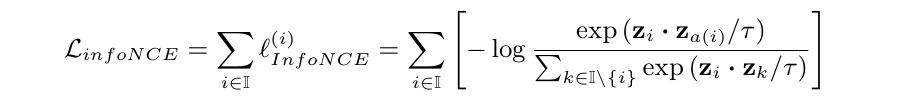
일반적으로 $x_i$를 anchor, $x_{a(i)}$를 positive, 나머지 샘플들을 negative라고 부른다. 결론적으로 infoNCE는 positive와의 거리는 가깝게, negative와의 거리는 멀게 하는 식으로 작동한다.

여기서 $g_B(x)$끼리 비교를 하는 것보다, projection layer $h_{\theta_{proj}}$를 통과해서 좀 더 저차원의 representation끼리 비교를 하는 게 좀 더 실용적이라고 한다. 따라서 $z_i=g_{B_t}(x_i)$를 $z_i=h_{\theta_{proj}}(g_{B_t}(x_i))$로 대체한다.

마지막으로, SCL(Supervised Contrastive Learning)이라는, infoNCE의 supervised 버전 변종을 고려한다. 한 anchor가 자신과 같은 클래스인 샘플을 여러개 가질 수 있으며, 따라서 SCL loss는 다음과 같다:

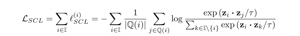
여기서 $\mathbb{Q}(i)$는 현재 anchor와 같은 클래스를 가진 샘플들을 말한다.

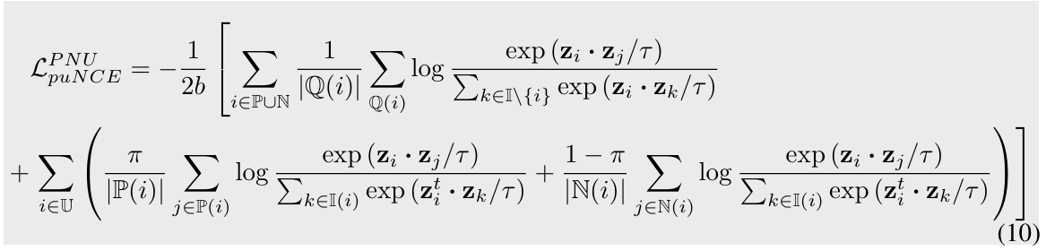
3. Positive Unlabeled NCE

---

그렇다면 이제 puNCE를 살펴볼 차례다.

puNCE의 핵심은 unlabeled sample이 $\pi$의 확률로 positive, $1-\pi$의 확률로 negative라고 가정하는 것이다.

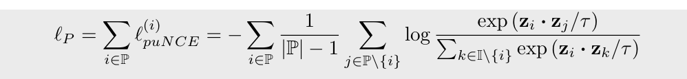
puNCE는 labeled anchor $x_i\in \mathcal{X}_P$에 대해, multi-viewed batch에 있는 다른 모든 labeled sample을 이 샘플과 최대한 가깝게 표현하고자 한다. (왜냐하면 labeled sample은 전부 positive이니까!)

multi-viewed batch $\tilde{\mathcal{D}}_t$에 대해, $\mathbb{P}\equiv\{k\in \mathbb{I}:s_k=1\}$을 labeled sample의 인덱스 집합, $\mathbb{U}\equiv\{k\in \mathbb{I}:s_k=0\}$을 unlabeled sample의 인덱스 집합이라 하자. puNCE의 labeled sample에 대한 empirical risk $\ell_P$는 다음과 같다:

다음으로, unlabeled anchor $x_i\in \mathcal{X}_U$는 확률 $\pi$에 따라 positive, negative 두가지 경우로 나뉜다.

1. positive로 가정한 경우: 모든 labeled sample + augmentation pair $x_{a(i)}$를 positive pair로 사용한다.
2. negative로 가정한 경우: negative labeled sample이 없기 때문에 오직 augmentation pair $x_{a(i)}$만 positive pair로 사용한다.

따라서 unlabeled sample에 대한 empirical risk $\ell_U$는 다음과 같다:

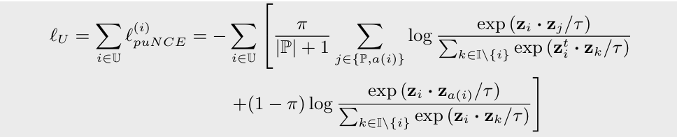
첫번째 부분은 positive로 가정한 경우, 두번째 부분은 negative로 가정한 경우에 대한 risk이다.

이 둘을 합치면 puNCE empirical risk는 다음과 같다:

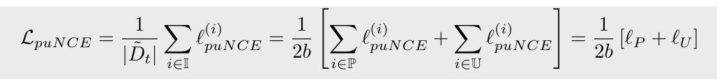
즉, puNCE는 모든 샘플에 각각 weight를 설정하는 것이다. 다시 말해서, labeled sample은 unit weight, unlabeled positive sample은 weight $\pi$, unlabeled negative sample은 weight $1-\pi$로 설정한다.

semi-supervised learning으로의 확장

semi-supervised learning에서 샘플은 positive, negative, unlabeled 세가지 종류가 있다(그래서 이를 PNU learning이라고도 부른다). 그렇다면, puNCE에서 unlabeled sample을 활용하는 방식을 여기에도 적용하는 것을 생각해볼 수 있다. 이 세팅에서 loss는 다음과 같은 형태를 가진다:

*supervised와 unsupervised의 경우에는 puNCE가 각각 SCL, infoNCE와 정확히 일치하므로 고려 대상이 아니다.

4. Experiments

---

4.1. Contrastive Positive Unlabeled Learning

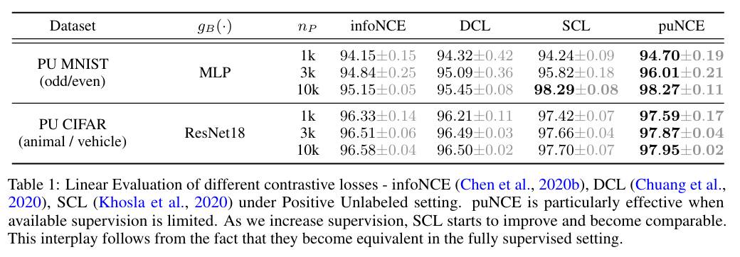
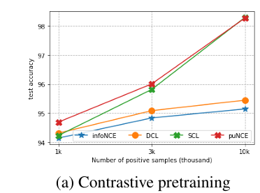
결과를 보면, $n_P$가 작을수록(즉, positive sample이 적을수록) puNCE가 상대적으로 강점을 갖게 되는 것을 확인할 수 있다.

4.2. Contrastive Positive Negative Unlabeled Learning

그렇다면 semi-supervised에선 어떨까?

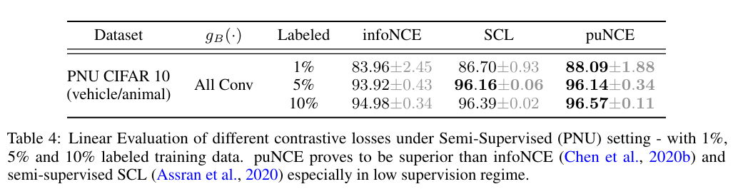
역시 puNCE가 뛰어났으며, 특히 10% 라벨의 경우 fully supervised baseline에 거의 근접했다고 한다.

4.3. PNU few shot learning

few-shot learning의 목표는 pretrained model을 약간의 labeled sample(few shot)만 사용해서 downstream task에 fine-tuning하는 것이다. few-shot learning에서 loss는 cross-entropy와 contrastive loss를 섞어서 사용한다.

puNCE는 여기에 추가로 unlabeled sample을 더 학습한다. 결과는 다음과 같다:

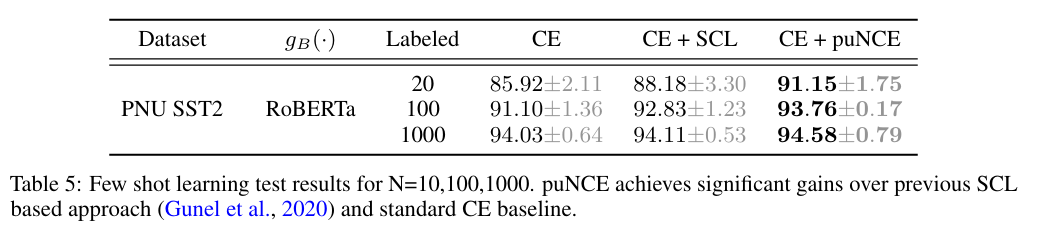
역시 puNCE가 가장 뛰어났다.

5. Conclusions

---

• puNCE는 contrastive loss를 PU 세팅으로 확장해서 weakly-supervised task에 보다 효율적으로 접근한다.
• puNCE는 PU, semi-supervised와 같이 supervision이 제한적인 세팅에서 기존 모델보다 뛰어난 성능을 보였다.