[Deep Learning] PyTorch로 인공신경망 모델 구축하기

Steven Lee·2023년 9월 16일

AI Deep Learning PyTorch

TRINITY

목록 보기

3/3

💡 지난 시간까지 공부한 다층 퍼셉트론의 구조를 적용해 간단한 인공신경망 모델 구측을 해보겠다. 라이브러리로는 PyTorch를 사용하였다.

사전 정보

(1) 사용 프로그램

Google Colab

(2) 예측할 모델

$y=\sqrt{x}$

(3) 사용 데이터

Input Data : x_train = [0,1,2,3,....999]
Actual Data : y_train = sqrt(x_train)
Learnin rate(학습률) : lr = 0.001
Epoch : 500
Batch size : 10
Loss Function : loss_fn = MSE
Optimizer : optimizer = Adam

🔥 x_train 데이터와 실제 예측 데이터인 y_train 데이터 두 개를 가지고 딥러닝을 이용하여 $y=\sqrt{x}$ 함수를 예측하고, 최종적으로 그래프까지 그림을 목적으로 한다.

1. Import Librarys

# Pytorch를 import
import torch
# 신경망 구축 시, 손실 함수와 레이어 단 같은 유용한 함수들을 가지는 라이브러리 import
import torch.nn as nn
# optimizer 기능을 손쉽게 사용하기 위해 import
import torch.optim as optim
# 행렬 연산을 도와주는 numpy import
import numpy as np
# 시각화를 도와주는 tool import
import matplotlib.pyplot as plt

2. Declare the Class - SqrtModel

# 1000x1 size의 tensor 생성 [0.; 1.; 2.;...999.;]
x_train = torch.arange(1000,dtype=float).unsqueeze(dim=-1)
# 예측 데이터와 비교할 실제 데이터(루트 함수에 x_train data 입력) tensor 생성
y_train = torch.sqrt(x_train)

# 구현시킬 모델 클래스 생성 - nn.Module을 상속 받는다
class SqrtModel(nn.Module) :
	
    # 객체가 갖는 속성값을 초기화하는 역할인, 생성자를 정의한다
    # 객체가 생성될 때 자동으로 호출되며, input과 output의 크기를 인수로 받게 된다.
	def __init__(self,input_size,output_size) :
    	# super을 호출해서 부모 클래스인 nn.Module의 속성들을 통해 
		# SqrtModel class를 초기화 한다.
        # super을 잘 모르겠으면 이 글을 참조하자 https://supermemi.tistory.com/179
    	super(SqrtModel,self).__init__()
        
        # 인수로 받은 input_size, output_size를 각 변수에 할당
        self.input_size = input_size
        self.output_size = output_size
        
        # 레이어 구성 설정
        self.layer = nn.Sequential(
        # Input Layer
        nn.Linear(self.input_size,10),
        # 배치 정규화 실행 -> 입력 데이터를 평균과 표준편차로 정규화(학습을 도움)
        nn.BatchNorm1d(10),
        # Activation 함수로 ReLU 함수 실행
        nn.ReLU(inplace=True),
		
        # Hidden Layer
        nn.Linear(10,30),
        nn.BatchNorm1d(30),
        nn.ReLU(inplace=True),
		
        # Output Layer
        nn.Linear(30,self.output_size)
    )
    
    # 모델이 학습데이터를 받아서 forward 연산을 수행하는 함수
    # model 객체를 데이터와 호출하면 자동으로 실행
    def forward(self,x):
    out = self.layer(x)
    return out

💡 $f(x)$ 식에 $x$ 로부터 예측된 $y$ 를 얻는 것을 forward 연산이라 한다.

3. Create an object of a class - model

# Sqrt 예측 모델 객체 생성(input_size : 1, output_size : 1)
model = SqrtModel(1,1)

4. HyperParameter Assignment

# Learning Rate(학습률)
lr = 0.001
# 반복 횟수
epoch = 500
# batch 사이즈
batch_size = 10
# 손실함수 선정 : MSE - 평균 제곱 오차 사용
loss_fn = nn.MSELoss()
# Optimizer 선정 : Adam 모델 사용
# model.parameters()는 업데이트되는 weight 값과 bias 값을 의미한다.
optimizer = optim.Adam(model.parameters(),lr)

5. Training

# epoch 값(횟수)만큼 학습을 진행(500번)
for epoch_cnt in range(epoch):
  # 입력 데이터를 shuffle 하는 코드 작성 
  # 랜덤하게 0~999까지를 배열한다.(ex. [1,43,999,...0]
  idx = torch.randperm(1000)
  
  # batch 값만큼씩 묶어서 학습 진행
  for batch_cnt in range(idx.shape[0]//batch_size):
  	# 랜덤으로 섞인 id 값인 idx에서 batch로 쓸 값들 slice (ex. [2,5,29,13,555,424,1,199,20,100])
    batch_indices = idx[batch_cnt*batch_size:(batch_cnt + 1)*batch_size]
    # batch 개수에 맞춰서 랜덤한 input 값들 추출
    batch = x_train[batch_indices,:]
    # batch 개수에 맞춰서 랜덤한 output 값들 추출
    target = y_train[batch_indices]
	
    # batch input을 넣고 sqrt 예측 모델의 forward 함수 실행 -> forward 연산 실행 -> 예측값 return
    predict = model(batch)
	
    # 예측 데이터와 진짜 데이터 간의 손실 값 측정(손실 함수 통해)
    loss = loss_fn(predict,target)
    # BackPropagation 실행
    loss.backward()
    # BackPropagation 통해 update된 weight, bias 값 반영
    optimizer.step()
	
    # 누적된 미분 값 초기화
    optimizer.zero_grad()

6. Test

# 모델을 학습 모드에서 평가 모드로 변환
model.eval()
# 우리가 만든 sqrt 모델에 넣을 9라는 값 할당
fake_data = torch.tensor([9],dtype=torch.float).unsqueeze(dim=0)

# 9를 넣고 sqrt모델 실행
out1 = model(fake_data)

>>> tensor([[2.9397]], grad_fn=<AddmmBackward0>)

7. Visualization

# autograd engine을 비활성화 시키고, 예측 모델에 train data 입력
with torch.no_grad():
    predicted_y = model(x_train)

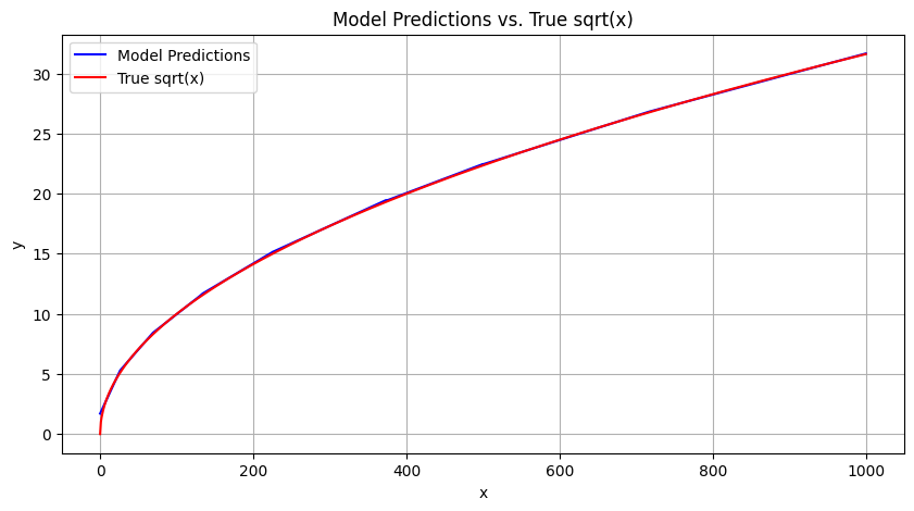
# matplotlib.pyplot을 이용한 데이터 visualization
plt.figure(figsize=(10, 5))
# 예측 모델은 파란색 그래프
plt.plot(x_train, predicted_y, label='Model Predictions', color='blue')
# 실제 sqrt 모델은 빨간색 그래프
plt.plot(x_train, torch.sqrt(x_train), label='True sqrt(x)', color='red')
plt.xlabel('x')
plt.ylabel('y')
plt.legend()
plt.title('Model Predictions vs. True sqrt(x)')
plt.grid()
plt.show()