
이 블로그글은 2019년 조재영(Kevin Jo), 김승수(SeungSu Kim)님의 딥러닝 홀로서기 세미나를 수강하고 작성한 글임을 밝힙니다.
Github 링크 : 실습 코드 링크
데이터를 Train, Valid, Test로 분리시키는 이유
Data Challnge
- Train : X, y가 주어짐
- Test : X가 주어짐
→ 성능을 확인할려면 Test의 X데이터를 통해 Pred y를 예측하고 제출하여 채점하는 방법밖에 없음
→ Train 데이터를 다시 Train 데이터와 Valid 데이터 셋으로 나눠서 Train 데이터로 학습하고 Valid 데이터로 평가
Pytorch Classification (Logistic Regression vs MLP)
💡 목표 : Classification Problem을 PyTorch로 해결해보기
Logistic Regression과 MLP를 둘 다 구현해보고 모델의 예측 데이터 분포를 시각화해서 MLP가 실제로 non-linear Decision-Boundary를 가질 수 있는지 살펴보자
# Pytorch 불러오기
import torch
print(torch.__version__)
# 나머지 모듈 불러오기
import numpy as np
import matplotlib.pyplot as plt데이터 생성 (정의)
데이터셋 설명
- discrete space에 분포하는 데이터
- 방사형 데이터 분포를 가상으로 만듦

데이터셋 정의
r = np.random.rand(10000) * 3
theta = np.random.rand(10000) * 2 * np.pi
y = r.astype(int)
r = r * (np.cos(theta) + 1)
x1 = r * np.cos(theta)
x2 = r * np.sin(theta)
X = np.array([x1, x2]).T
데이터셋 split (훈련, 검증, 테스트)
train_X, train_y = X[:8000, :], y[:8000]
val_X, val_y = X[8000:9000, :], y[8000:9000]
test_X, test_y = X[9000:, :], y[9000:]
💡 참고
pytorch에서 데이터 셋은 첫 번째 차원은 샘플의 개수를 나타내도록 설계되어 있음
데이터셋 시각화
# 데이터셋 시각화
fig = plt.figure(figsize=(12, 5))
ax1 = fig.add_subplot(1, 3, 1)
ax1.scatter(train_X[:, 0], train_X[:, 1], c=train_y, s=0.7)
ax1.set_xlabel('x1')
ax1.set_ylabel('x2')
ax1.set_title('Train set Distribution')

ax2 = fig.add_subplot(1, 3, 2)
ax2.scatter(val_X[:,0], val_X[:,1], c=val_y)
ax2.set_xlabel('x1')
ax2.set_ylabel('x2')
ax2.set_title('Validation set Distribution')

ax3 = fig.add_subplot(1, 3, 3)
ax3.scatter(test_X[:,0], test_X[:,1], c=test_y)
ax3.set_xlabel('x1')
ax3.set_ylabel('x2')
ax3.set_title('Test set Distribution')

plt.show()
Hypothesis 정의 (모델 정의)
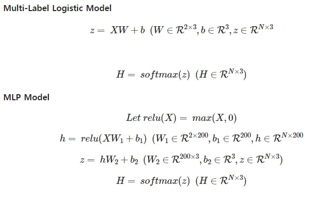
Multi-Label Logistic Model (Linear Model)
- (주의) Model 내에서 Softmax 사용할 필요없이 뒤에 CrossEntropyLoss 함수 안에 Softmax 함수가 있기 때문
- PyTorch의
nn.module을 상속받아 새로운 신경망 모델 클래스를 정의 __init__은 클래스 초기화 메서드 (생성자)- super를 통해 부모 클래스의 초기화를 호출하여 상속받은 속성들을 초기화
- 선형 레이어 정의
- 입력 크기 : 2, 출력 크기 : 3, bias가 있음
forward는 입력 x를 받아 선형 변환을 적용하는 출력값을 반환하는 메서드
import torch.nn as nn
class LinearModel(nn.Module):
  def __init__(self):
    super(LinearModel, self).__init__()
    self.linear = nn.Linear(in_features=2, out_features=3, bias=True)

  def foward(self, x):
    return self.linear(x)
MLPModel
- 마찬가지로 이후에 CrossEntropyLoss함수를 적용하면 되므로 Regression 문제를 풀 때와 똑같은 모델 생성
- PyTorch의
nn.Module을 상속받아 다층 퍼셉트론 모델 클래스를 정의 __init__은 클래스 초기화 메서드(생성자)- super를 통해 부모 클래스의 초기화를 호출하여 상속받은 속성들을 초기화
- 첫 번째 선형 레이어 정의
- 입력 크기 : 2, 출력 크기 : 200
- 두 번째 선형 레이어 정의
- 입력 크기 : 200, 출력 크기 : 3
- 활성화 함수로 ReLU 정의
forward는 입력 x를 받아 순전파(forward pass)를 수행하는 메서드- 첫 번째 선형 레이어를 통해 입력을 변환
- 변환된 값에 ReLU 활성화 함수를 적용하여 비선형성을 추가
- 두 번째 선형 레이어를 통해 최종 출력을 생성하고 반환
class MLPModel(nn.Module):
	def __init__(self):
		super(MLPModel, self).__init__()
		self.linear1 = nn.Linear(in_features=2, out_features=200)
		self.linear2 = nn.Linear(in_features=200, out_features=3)
		self.relu = nn.ReLU()

	def forward(self, x):
		x = self.linear1(x)
		x = self.relu(x)
		x = self.linear2(x)
		return x
Cost Function 정의
- Pytorch의 nn 모듈에 구현된 CrossEntropyLoss 사용
- 주의할것이 input은
N X NumClass차원을 가지는 float 형태여야하고 target은N차원을 가지고 각 엘리멘트의i번째 클래스를 나타내는 int형이여야함
cls_loss = nn.CrossEntropyLoss()학습 및 평가
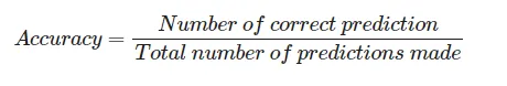
- 이번에는 최종적인 모델에 test를 위해 Accuracy를 metric으로 사용함
모델 생성
import torch.optim as optim
from sklearn.metrics import accuracy_score

#**model = LinearModel()
#print(model.linear.weight)
#print(model.linear.bias)**

model = MLPModel()
print(f'{sum(p.numel() for p in model.parameters() if p.requires_grad)} Parameters')
Optimizer 생성
lr = 0.005
optimizer = optim.SGD(model.parameters(), lr=lr)
학습 & 검증
Train 부분
list_epoch = []
list_train_loss = []
list_val_loss = []
list_mae = []
list_mae_epoch = []
epoch = 4000
for i in range(epoch):
# Trian
model.train()
optimizer.zero_grad()
input_x = torch.Tensor(train_X)
true_y = torch.Tensor(train_y).long()
pred_y = model(input_x)
loss = cls_loss(pred_y.squeeze(), true_y)
loss.backward()
optimizer.step()
list_epoch.append(i)
list_train_loss.append(loss.detach().numpy())
# Validate
model.eval()
optimizer.zero_grad()
input_x = torch.Tensor(val_X)
true_y = torch.Tensor(val_y).long()
pred_y = model(input_x)
loss = cls_loss(pred_y.squeeze(), true_y)
list_val_loss.append(loss.detach().numpy())
if i % 200 == 0:
model.eval()
optimizer.zero_grad()
input_x = torch.Tensor(test_X)
true_y = torch.Tensor(test_y).long()
pred_y = model(input_x).detach().max(dim=1)[1].numpy()
mae = mean_absolute_error(true_y, pred_y)
list_mae.append(mae)
list_mae_epoch.append(i)
fig = plt.figure(figsize=(15,5))
ax1 = fig.add_subplot(1, 3, 1, projection='3d')
ax1.scatter(test_X[:, 0], test_X[:, 1], test_y, c=test_y, cmap='jet')
ax1.set_xlabel('x1')
ax1.set_ylabel('x2')
ax1.set_zlabel('y')
ax1.set_zlim(-10, 6)
ax1.view_init(40, -40)
ax1.set_title('True test y')
ax1.invert_xaxis()
ax2 = fig.add_subplot(1, 3, 2, projection='3d')
ax2.scatter(test_X[:, 0], test_X[:, 1], pred_y, c=pred_y[:,0], cmap='jet')
ax2.set_xlabel('x1')
ax2.set_ylabel('x2')
ax2.set_zlabel('y')
ax2.set_zlim(-10, 6)
ax2.view_init(40, -40)
ax2.set_title('Predicted test y')
ax2.invert_xaxis()
input_x = torch.Tensor(train_X)
pred_y = model(input_x).detach().numpy()
ax3 = fig.add_subplot(1, 3, 3, projection='3d')
ax3.scatter(train_X[:, 0], train_X[:, 1], pred_y, c=pred_y[:,0], cmap='jet')
ax3.set_xlabel('x1')
ax3.set_ylabel('x2')
ax3.set_zlabel('y')
ax3.set_zlim(-10, 6)
ax3.view_init(40, -40)
ax3.set_title('Predicted train y')
ax3.invert_xaxis()
plt.show()
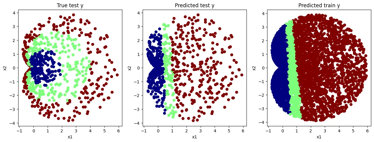
print(i, loss)Multi-Label Logistic Model (Linear Model)
- 직선으로 밖에 분류를 못하므로 결과가 제대로 나오지 않음
- Non-Linear한 decision boundary를 만들지 못함
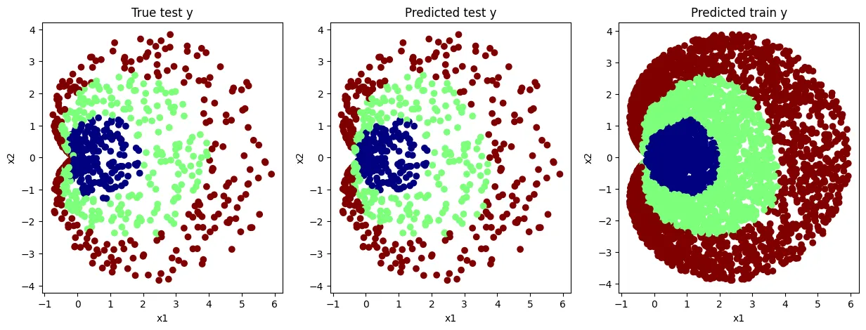
MLP Model
- Non-Linear한 decision boundary를 만들어냄
결과
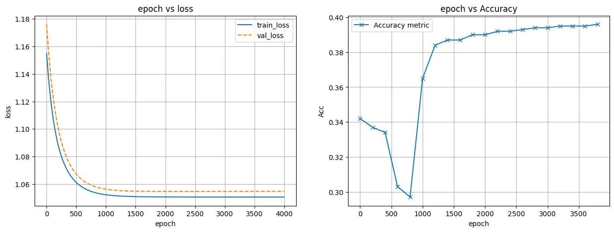
Multi-Label Logistic Model (Linear Model)
- accuracy 성능이 50%를 체 못 넘긴다. (크게 분별력을 가지는 모델을 만들지 못함)
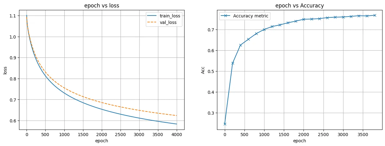
MLP Model
- accuracy 성능이 76% 정도인 모델을 만듦

제 글이 유익하셨다면 ♡와 팔로우로 응원 부탁드립니다.