[ML] 5주차-1 : Cost Function and Backpropagation

Machine Learning by professor Andrew Ng in Coursera

1) Cost Function

Neural Network (Classification)

---

우선 앞으로 사용할 새로운 변수들

• L = total no. of layers in network
• $s_l$ = no. of units (not counting bias unit) in layer $l$

Binary Classification에서 y는 0 또는 1 만을 갖는다.
즉, output unit은 1개 &

Multiclass Classification (K classes) 라면
output units은 K개 &

Cost Function

---

neural network는 많은 ouput nodes를 가질 수 있다.
이때 $h_\Theta(x)_k$를 $k$번째 $output$의 $hypothesis$라고 한다.
Our cost function for neural networks is going to be a generalization of the one we used for logistic regression. Recall that the cost function for regularized logistic regression was:

Logistic Regression:

Neural Network:

'이때 regularization term들은 전부 0이 아니라 1부터 $\sum$ 가 시작된다.
bias term $\theta_0$는 정규화하지 않기 때문'

• multiple output nodes를 고려하기 위해 몇 개의 nested summation이 추가된다.
  • 대괄호([ ]) 안에 output node 갯수만큼 반복되는 nested summation이 추가된다.
• 정규화 부분에서 multiple theta 행렬을 고려해야 한다.
  • theta 행렬의 열은 bias unit을 포함한 현재 layer의 node 개수와 같다.
  • theta 행렬의 행은 bias unit을 제외한 다음 layer의 node 개수와 같다.
  • logistic regression과 마찬가지로 모든 항을 제곱한다.

2) Backpropagation Algorithm

"Backpropagation"은 neural-network에서 비용 함수의 최솟값을 찾는 방법으로 logistic/linear regression에서의 gradient descent와 같은 역할을 한다.

Gradient Computation

---

비용 함수를 최소화하는 최적의 parameter $\theta$ 찾아야 한다.
즉,

$J(\theta)$는 이미 위에서 알았고,
$\frac{\partial}{\partial \Theta_{i,j}^{(l)}} J(\Theta)$를 어떻게 계산할지 알아본다.

Given one training example (x, y):

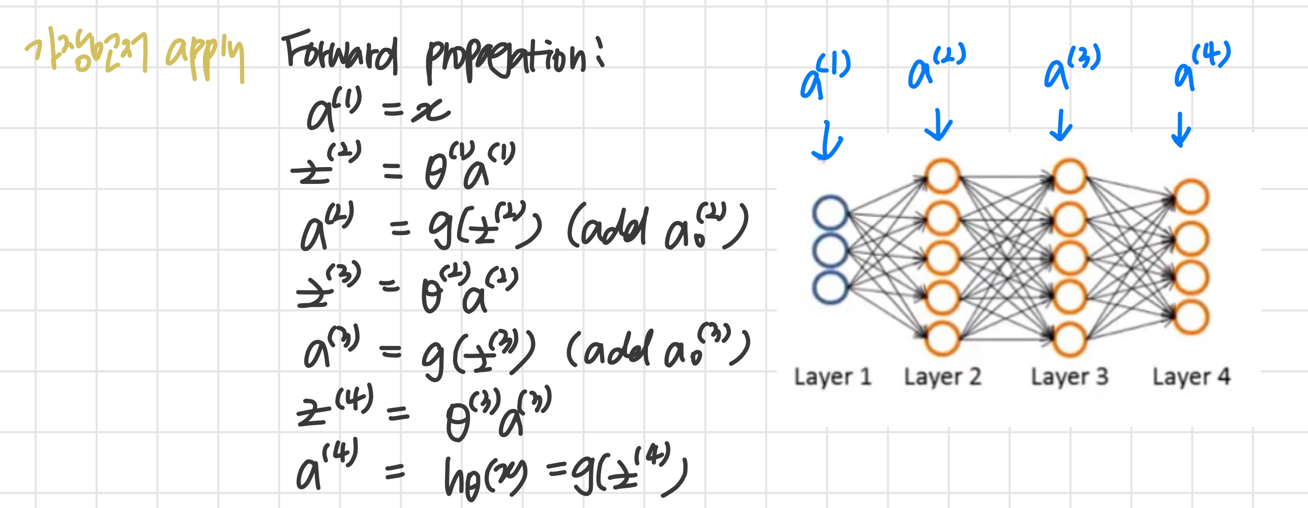
Gradient Computation : Backpropagation algorithm

---

• $\delta_j^{(l)}$ = $error$ of node $j$ in layer $l$
  

Backpropagation algorithm

---

$\{((x^{(1)}, y^{(1)}) ... (x^{m}, y^{(m)})\}$ 의 훈련세트가 주어진다.

• $\delta_{ij}^{(l)} = 0 \text{ (for all l, i, j)}$ 라 설정한다.

For i=1 to m

1. Set $a^{(1)}:= x^{(i)}$

2. Perform forward propagation to compute $a^{(l)} \text{ for l = 1, 2, ... L}$

3. $y^{(i)}$를 이용해서 $\delta^{(L)} = a^{(L)} - y^{(i)}$을 계산한다.

4. $\delta^{(l)} = ((\Theta^{(l)})^T\delta^{(l+1)}).*a^{(l)}.*(1-a^{(l)})$ 을 이용해서 $\delta^{(L-1)}, \delta^{(L-2)}... \delta^{(2)}$를 계산한다.

이때 .*은 element-wise multiply 를 의미한다.
$g'(z^{(l)}) = a^{(l)} .* (1-a^{(l)})$

5. $\Delta_{i, j}^{(l)} := \Delta_{i, j}^{(l)} + a_j^{(l)}\delta_i^{(l+1)}$, 이 식을 벡터화하면 $\Delta^{(l)} := \Delta^{(l)} + \delta^{(l+1)}(a^{(l)})^T$

for 루프를 빠져나온 뒤
새로운 $\Delta$ 행렬을 아래와 같이 업데이트한다.

• $D_{i, j}^{(l)} := \frac{1}{m}(\Delta_{i, j}^{(l)}+\lambda\Theta_{i, j}^{(l)}), \text{ if j}\neq0$

• $D_{i, j}^{(l)} := \frac{1}{m}\Delta_{i, j}^{(l)}, \text{ if j}\equiv0$

이렇게 $D_{ij}^{(l)}$을 계산하면

그게 곧 $\dfrac{\partial J(\Theta)}{\partial \Theta_{i,j}^{(l)}} = D_{i,j}^{(l)}$

The capital-delta matrix D is used as an "accumulator" to add up our values as we go along and eventually compute our partial derivative.
$D$ 행렬은 결국에는 편미분을 구하게 해주는 "accumulator"로 동작한다.

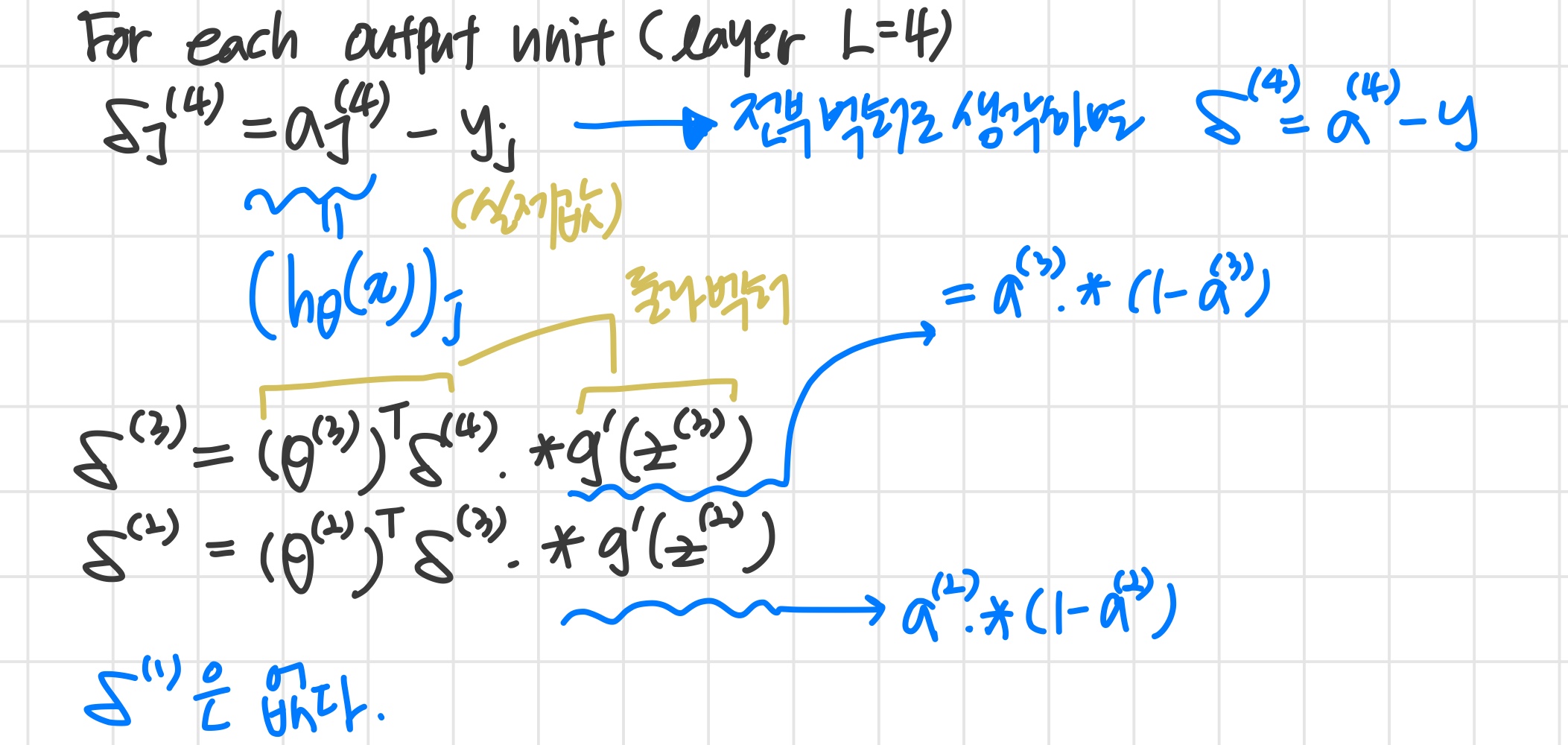
3) Backpropagation Intuition

Forward Propagation

---

What is backpropagation doing?

---

neural network의 cost function은 아래와 같다.

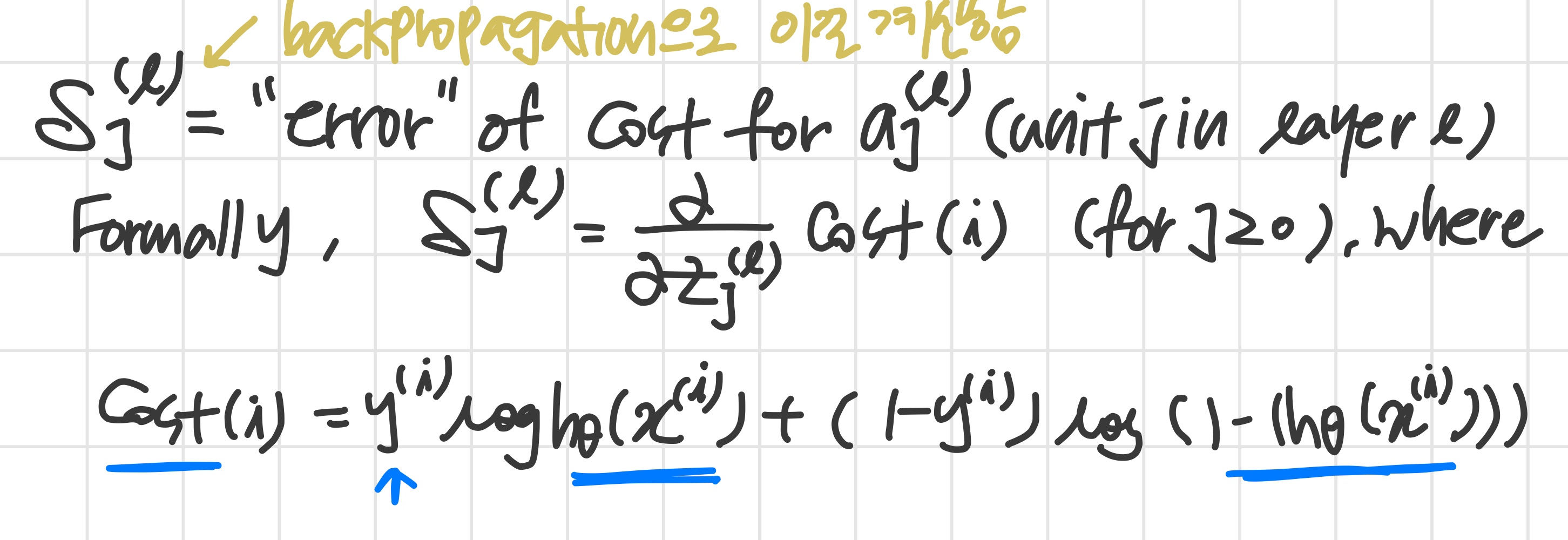
If we consider simple non-multiclass classification (k = 1) and disregard regularization, the cost is computed with:

Intuitively, $\delta_j^{(l)}$ is the "error" for $a_j^{(l)}$ (unit j in layer l). More formally, the delta values are actually the derivative of the cost function:

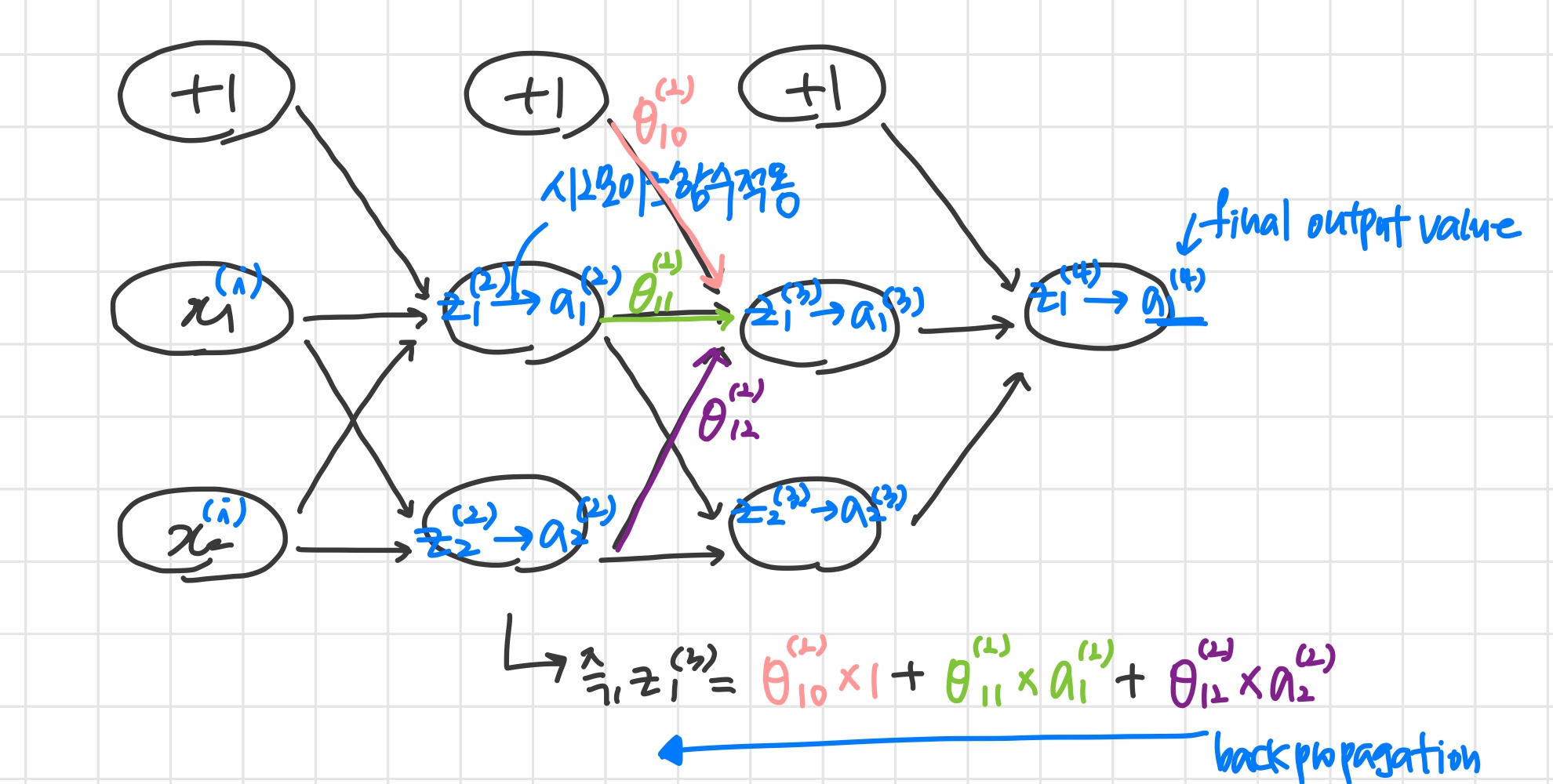
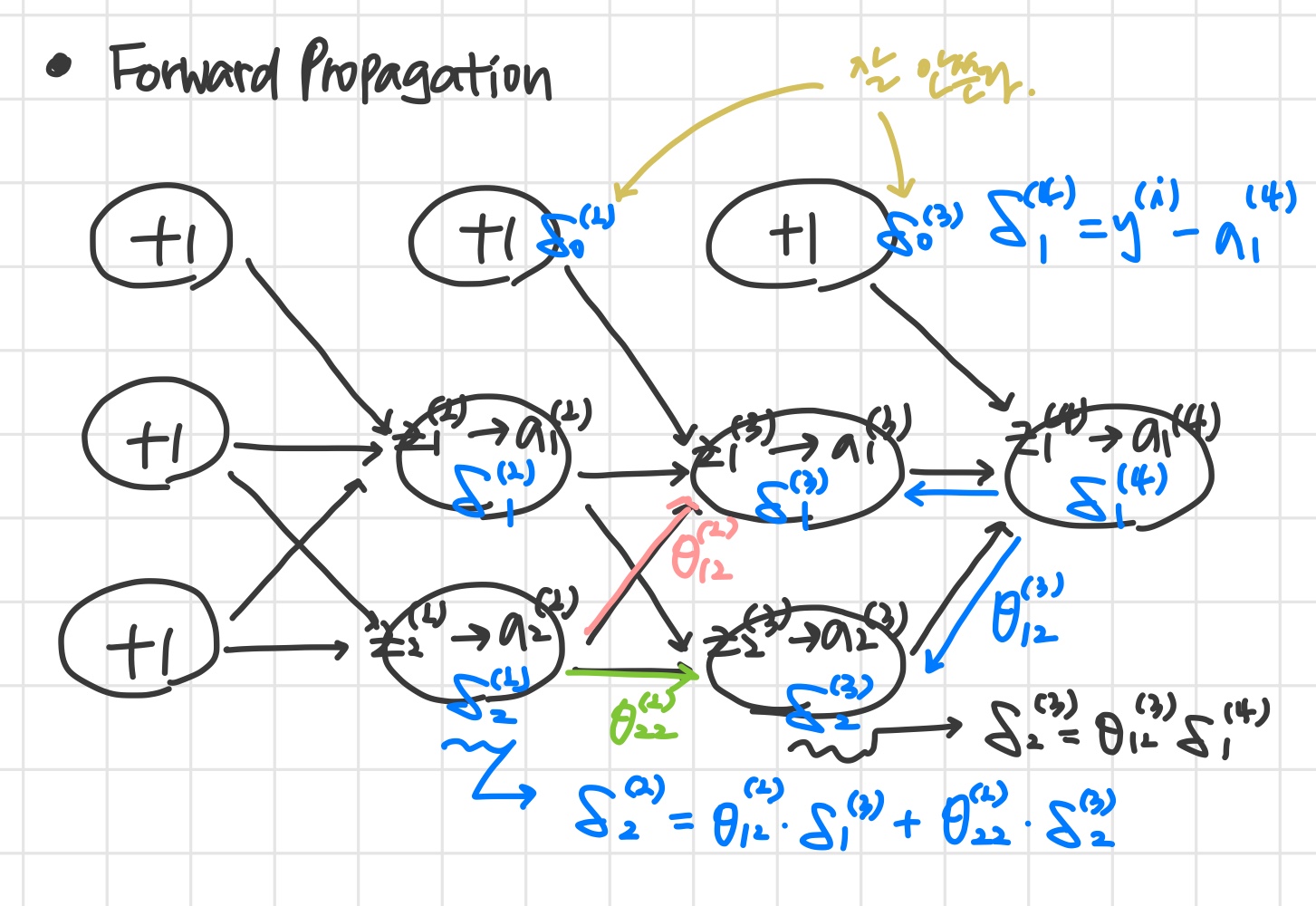
Recall that our derivative is the slope of a line tangent to the cost function, so the steeper the slope the more incorrect we are. Let us consider the following neural network below and see how we could calculate some $\delta_j^{(l)}$:

_😡