[ML] 5주차-2 : Backpropagation in Practice

Machine Learning by professor Andrew Ng in Coursera

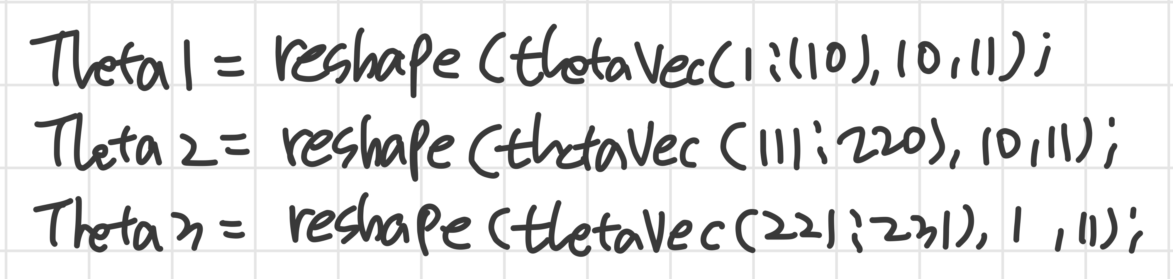
1) Implementation Note: Unrolling Parameters

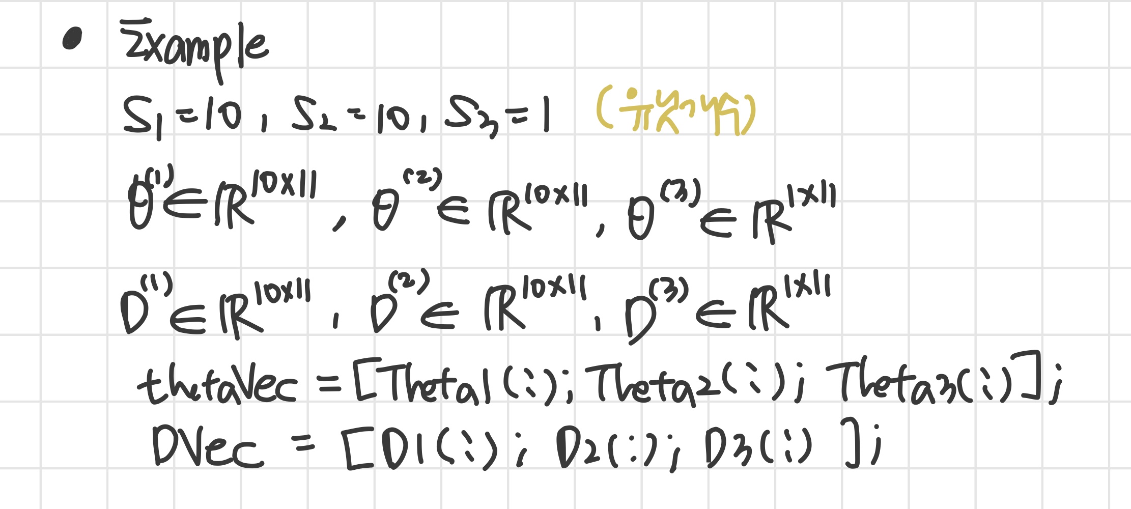
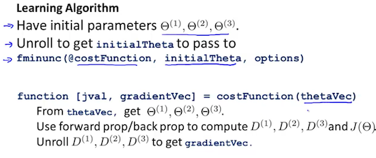
'이전에 언급한 advanced optimization 방법에서는 unrolled 형태가 필요할 수 있다. 그럴때 이 방법을 쓴다.'

2) Gradient Checking

'backpropagation이 잘 작동하고 있는지 확인할 수 있다.'

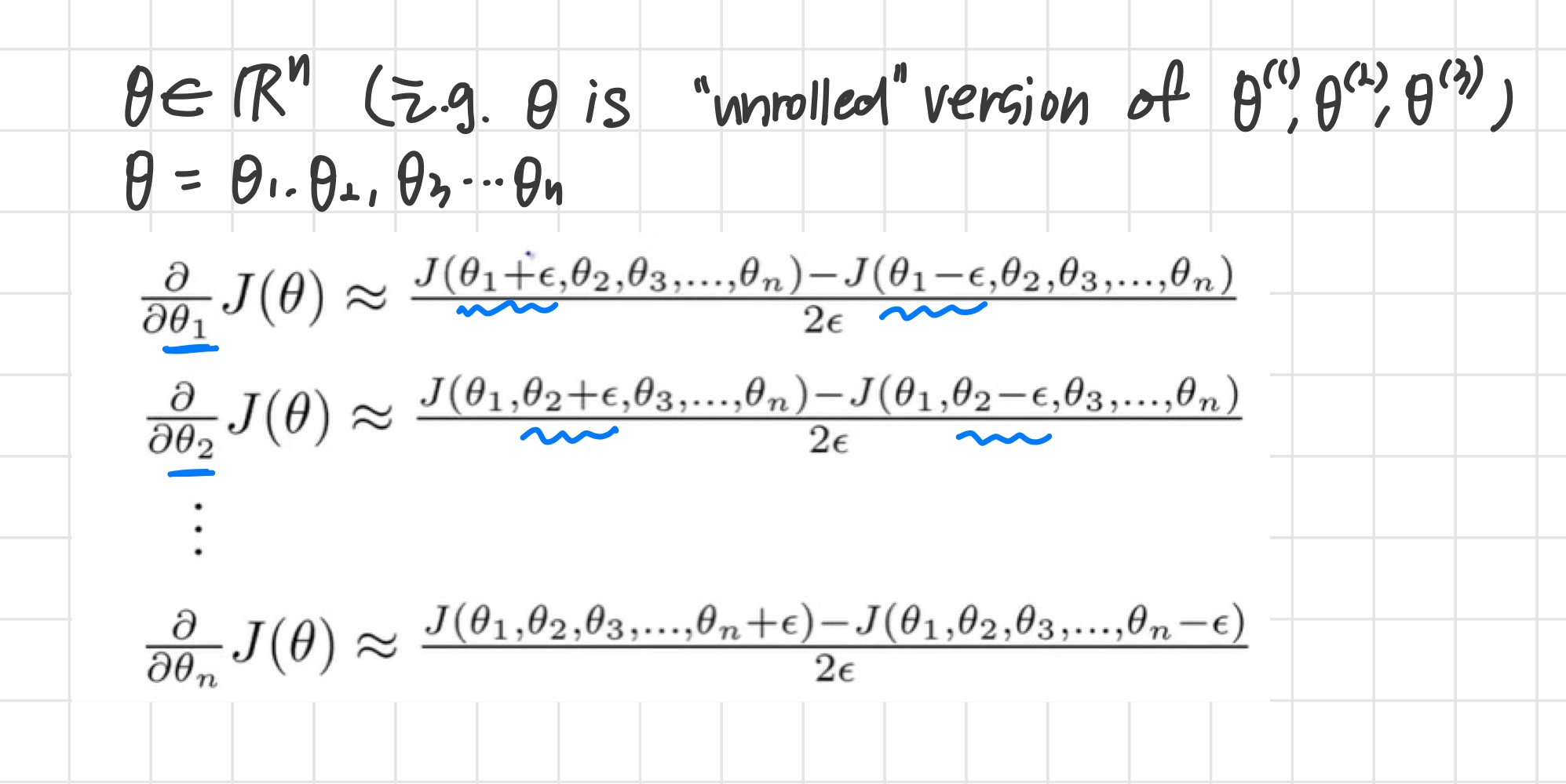
Numerical estimation of gradients

---

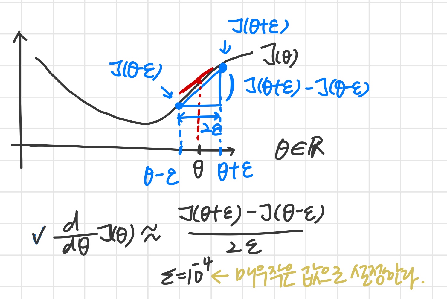
We can approximate the derivative of our cost function with:

두 식의 값은 비슷해야 한다.

Parameter Vector $\theta$

---

이때 주의할 점
$\dfrac{\partial}{\partial \Theta}J(\Theta)$와 numerical estimation이 서로 유사한 값을 가지는 것을 확인한 뒤 (즉, backpropagation algorithm이 제대로 작동하고 있는 것을 확인한 뒤)
분류기를 실제로 훈련시킬 때, gradient checking 코드를 반드시 disable 해줘야 한다.
그렇지 않으면 속도가 매우 느려진다.

3) Random Initialization

Initial value of $\Theta$

---

gradient descent와 advanced optimization 방법을 사용하려면 $\Theta$의 초깃값을 설정해줘야 한다.

Zero initialization

---

$\Theta$의 초깃값을 전부 0으로 설정한 경우

• $a_1^{(2)} = a_2^{(2)}$
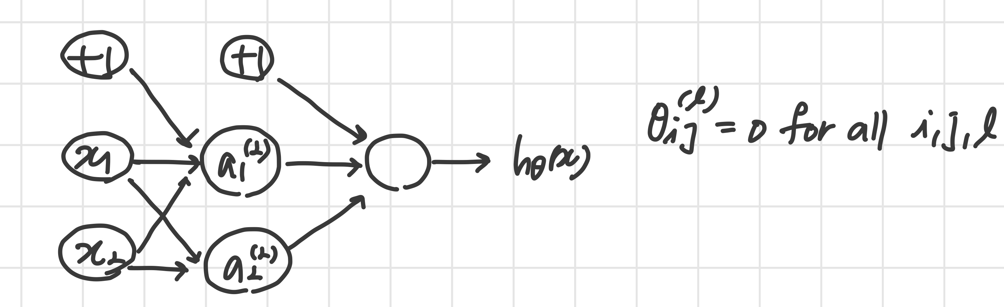
• $\Theta$가 전부 0이기 때문에 또한 $\delta_1^{(2)} = \delta_2^{(2)}$
• $\dfrac{\partial}{\partial \Theta_{01}^{(1)}}J(\Theta) = \dfrac{\partial}{\partial \Theta_{02}^{(1)}}J(\Theta)$ 즉, $\Theta_{01}^{(1)} = \Theta_{02}^{(1)}$
• 같은 입력단에서 나온 weight들에는 같은 값이 들어간다.

'즉 x1 유닛에서 나오는 값은 모두 같고, x2 유닛에서 나오는 값은 모두 같다.'
따라서 전부 0으로 초기화하면 안 된다.
랜덤값으로 초기화해줘야 한다.

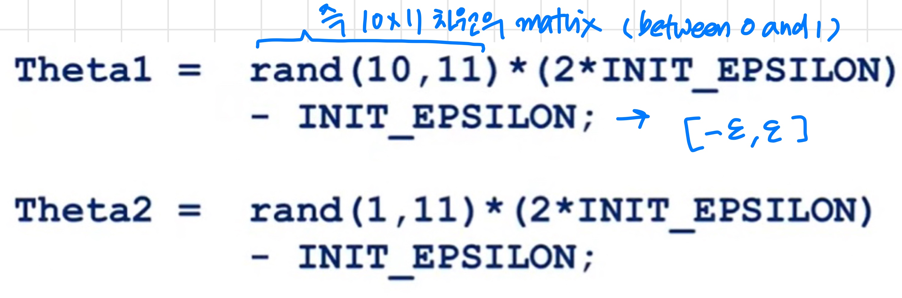
Random initialization : Symmetry breaking

---

각 $\Theta_{ij}^{(l)}$을 $[-\epsilon, \epsilon]$ 인 랜덤값으로 초기화한다.

4) Putting it together

지금까지 배운 것들 전부 정리
우선 network 구조를 고른다.
각 layer의 hidden unit 개수, 총 몇 개의 layer를 둘 지와 같은 neural network의 layout을 결정한다.

• input unit 개수 : dimension of features $x^{(i)}$
• output unit 개수 : class 개수
• layer 당 hidden unit 개수 : 많을수록 좋다. (hidden unit이 많아질수록 must balance with cost of computation)
• Defaults : hidden layer 1개. 만약 hidden layer가 1개 이상이라면 각 hidden layer에 같은 unit 개수를 두는 것이 권장된다.

Training a neural network

---

1. weights를 랜덤하게 초기화한다.
2. $h_\theta(x^{(i)})$를 구하기 위해 모든 $x^{(i)}$에 대해 forward propagation을 계산한다.
3. 비용 함수를 계산한다.
4. partial derivative $\dfrac{\partial}{\partial \Theta_{jk}^{(l)}}J(\Theta)$를 구하기 위해 backpropagation을 계산한다.
5. gradient checking을 통해 backpropagation이 잘 작동하는지 확인한다. ('값이 유사한지 확인') 확인 후 gradient checking을 disable한다.
6. Use gradient descent or a built-in optimization function to minimize the cost function with the weights in theta.

The following image gives us an intuition of what is happening as we are implementing our neural network:

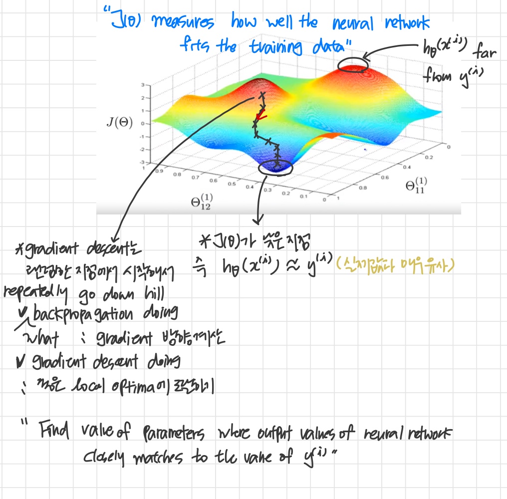
However, keep in mind that $J(\Theta)$ is not convex and thus we can end up in a local minimum instead.