Logistic Regression

---

• 몇개의 regression algorithm중 logistic regression은 classification문제에서도 사용할 수 있다.

• logistic regression은 sample이 특정 class에 속할 확률을 추정하여 positive class, negative class를 predict하는 binary classification에 사용된다.

1. Estimate probabilities

---

• Logistic regression model은 linear regression처럼 input feature와 weights의 linear combination($w^T\cdot x$)를 계산하지만 이를 바로 출력 하는 것이 아니라 logistic을 output으로 갖는다.
  
  

* probability estimation of logistic regression

• 위의 수식중 $\sigma(\cdot)$은 0과 1 사이의 값을 출렷하는 sigmoid함수로 아래와같은 식과 그래프로 나타난다.

* logistic function (sigmoid function)

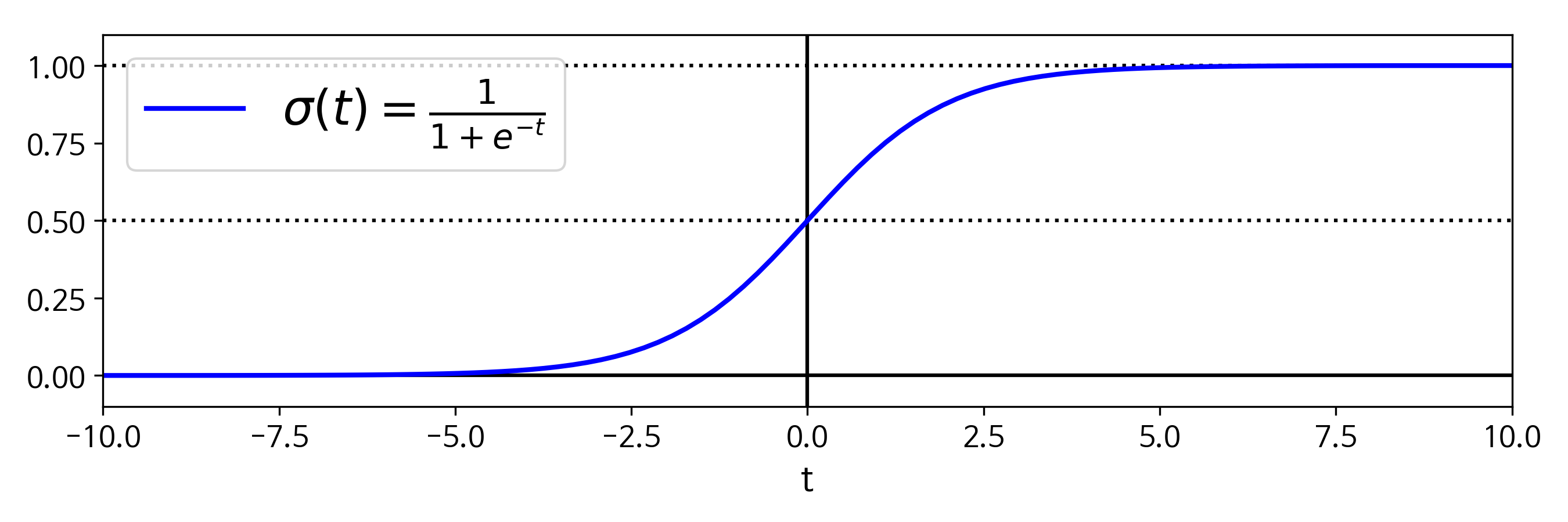
• 위 수식에서 t < 0 이면 $\sigma(t)$ < 0.5 이고 t > 0 이면 $\sigma(t)$ > 0.5 가 되므로 logistic model은 $\theta^T\bold{x}$ 가 양수일때 1 (positive class) 음수일때 0 (negative class)로 예측하게된다.

2. Training and Cost Function

---

• Logistic regression model 훈련의 목적은 positive class에는 높은 확률은 추정하고 negative class에는 낮은 확률을 추정하는 weights($\theta$)를 찾는 것 이다.

• 이러한 idea로 하나의 sample에 대한 loss function은 다음과 같은 수식으로 나타난다.

* 참고용

• 하나의 smaple에 대한 loss function을 나타내는 위 수식은 $\hat{p}$이 0에 가까워질수록 $-log(\hat{p} )$가 무한대로 커지는 형태로 model이 해당 sample을 0에 가까운 확률로 추정한다면 loss가 매우 커지는 것으로 볼 수 있고

• $\hat{p}$가 0에서 1에 가까워 질 수록 $-log(1-\hat{p} )$가 0에 가까워지는 형태로 model이 해당 sample을 1에 가까운 확률로 추정한다면 loss는 0에 가까운 값이 된다는 것을 나타낸다.

• 전체 training set에 대한 loss function은 모든 sample의 loss를 평균낸 것으로 수식은 다음과같이 나타낸다.

* Logistic Regression cost function (log loss)

• 이 loss function은 normal equation같이 최솟값을 계산하는 해가 없다. 하지만 이 loss function은 convex function이므로 global minimum에 도달하기 위한 theoretical guarantees를 제공한다.

• 위 식은 sample이 positive class ($y^{(i)}=1$)이면 ($1-y^{(i)}= 0$)이 되어 $y^{(i)}log(\hat{p}^{(i)})$만 남게되고 negative class ($y^{(i)}=0$)이면 $log(1-\hat{p}^{(i)})$ 만 남게되는 형태로 이전에 보았던 하나의 sample에 대한 loss function 이 일반화된 형태이다.
  

• 이 loss function에 대한 편도함수는 다음과 같다.

• 이러한 편도함수를 모든 $\theta_j ~ (w_j)$에 대하여 구하면 gradient vector로서 gradient descent 에 사용할 수 있게 된다.

3. Decision Boundaries

---

• 앞에서 logistic regression은 classification문제에 활용할 수 있다고 하였는데 그 예를 sklearn의 붓꽃 데이터셋으로 살펴보자.

from sklearn import datasets

iris = datasets.load_iris()
print(iris.keys())
print('feature_names : ',iris['feature_names'])
print('target_names : ',iris['target_names'])

'''
dict_keys(['data', 'target', 'target_names', 'DESCR', 'feature_names', 'filename'])
feature_names :  ['sepal length (cm)', 'sepal width (cm)', 'petal length (cm)', 'petal width (cm)']
target_names :  ['setosa' 'versicolor' 'virginica']
'''

• iris dataset은 위와같은 feature와 target data를 가지고있다.

import numpy as np

X = iris['data'][:,3:]  # petal width (cm)
y = (iris['target'] == 2).astype(np.int)  # virginica (target)

• 꽃잎의 너비(petal width)를 기반으로 target class중 하나인 virginica 종을 감지하는 classifier를 생성해보자.

import matplotlib.pyplot as plt

X_new = np.linspace(0, 3, 1000).reshape(-1, 1)
y_proba = log_reg.predict_proba(X_new)

decision_boundary = X_new[y_proba[:, 1] >= 0.5][0]

plt.plot(X[y==0], y[y==0], "bs")  # virginica (초록세모)
plt.plot(X[y==1], y[y==1], "g^")  # not virginica (another iris) (파란네모)
plt.plot([decision_boundary, decision_boundary], [0, 1], "k:", linewidth=2)  
plt.plot(X_new, y_proba[:,1], 'g', label='Iris virginica')  # virginica (초록실선)
plt.plot(X_new, y_proba[:,0], 'b--', label='Not Iris virginica') # not virginica (파란점선)
plt.text(decision_boundary+0.02, 0.15, "decision boundary", fontsize=11, color="k", ha="center")
plt.arrow(decision_boundary, 0.08, -0.3, 0, head_width=0.05, head_length=0.1, fc='b', ec='b')  # 초록(virginica) 화살표
plt.arrow(decision_boundary, 0.92, 0.3, 0, head_width=0.05, head_length=0.1, fc='g', ec='g')  # 파란(not virginica) 화살표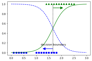

• 위 그림은 0~3(cm) 범위의 1000개의 petal width값을 학습시킨 Logistic regression model을 통해 predict 하여 그래프로 나타낸 그림이다. 그냥 virginica 와 not virginica에 대한 학습시킨 probabilites function이라고 보면된다.

• 초록 세모와, 파란 네모는 0~3(cm) 범위안의 petal width크기에 대한 target label로 각 virginica와 not virginica이다.

• 위 그림에서 보다시피 virginica class는 petal width가 약 1.4 ~ 2.5에 분포하며 (초록세모), other class는 0.1 ~ 1.8에 분포한다. 이때 범위가 중첩되는 부분인 1.6 근처에서 decision boundary가 생기게 된다.

• 이때 logistic regression은 linear regression의 decision boundary에서 생기는 문제를 확률적으로 접근하여 해결하게 되는 것이다.

• 이번엔 두개의 특성을통해 학습된 model의 decision boundary를 살펴보자.

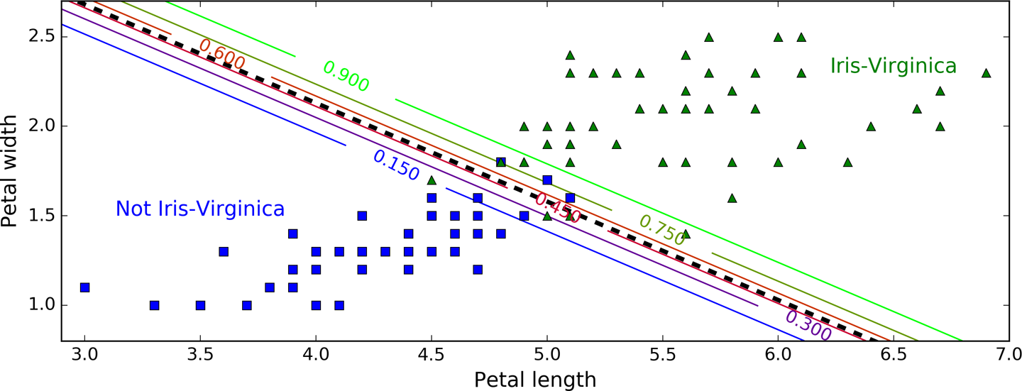
• 위 그림은 petal width, petal length 두 feature를 학습시킨 결과이다.

• 가운데 검은 점선은 model이 50% 확률을 추정하는 지점으로 해당 model의 decision boundary이며, 부근의 직선들은 model이 15% ~ 90% 확률을 출력하는 point를 나타낸다. 맨 오를쪽 위의 연두색 직선을 넘어선 data들은 model이 90% 확률로 virginica로 판단한다는 것이다.

4. Softmax regression

---

• softmax regression은 다른말로 multinorminal logistic regression으로 logistic regression의 binary classifier
  를 multiclass에 대해 지원하도록 일반화 시킨 것이다.

• 주어진 sample에 대해 model이 각 클래스 k에 대한 점수 $s_k \bold{(x)}$를 계산하고 이 점수에 softmax function(normalized exponential function)을 적용하여 각 클래스의 확률을 추정하는 형태이다.

* Softmax score for class k

• 각 클래스마다 해당 weights vector $\theta^k$를 가지고있고 이 vector들은 parameter matrix에 row vector로 저장된다.

• sample $\bold{x}$에 대해 각 클래스별 점수를 계산 후 softmax function을 취해주어 클래스 k 에 속할 확률 $\hat{p}_k$를 계산하게된다.

• softmax function 은 다음과 같다.

* Softmax function

- $k$ : num of classes.
- $s(x)$ : sample $\bold{x}$에 대한 각 클래스의 점수를 담은 vector.
- $σ(s(\bold{x}))_k$ : smaple x가 k에 속할 확률 추정값(estimated probability) .

• logistic regression과 마찬가지로 softmax regression는 다음 식처럼 estimated probability인 score가 가장 높은 클래스를 선택한다.

* Softmax Regression classifier prediction

• argmax 연산은 함수를 최대화하는 변수의 값을 반환한다. 이 식에서는 estimated probability인 $σ(s(\bold{x}))_k$의 최대인 k를 반환한다.
  
  

* softmax regression classifier는 multiclass classifier이지 multioutput classifier가 아니기에 한번에 하나의 클래스만 예측 할 수 있고, iris data처럼 mutually exclusive(상호 베타적인) classes 에서만 사용할 수 있다.

• model이 estimated probability를 계산하는 방법을 보았으니 어떻게 학습하는지 알아보자.

• softmax regression train의 핵심은 target class에는 높은 확률을 other class에는 낮은 확률을 계산하도록 만드는 것이다.

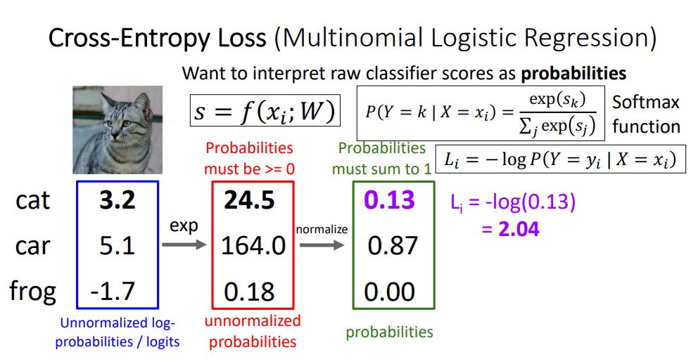
* Cross entropy loss function

• 위 수식은 cross entropy loss를 일반화시킨 형태의 function으로 class 하나에 대한 cross entropy loss는 단순히 아래의 수식처럼 softmax function에 -log를 취해주는 것 이다.

• 위 수식에 의하여 loss를 구하게되는 방식을 풀면 다음과 같다.

  1. 각 class별 score ($s_k(\bold{x})$)에 exponential을 취하여 양수값을 갖게한다.

  2. 각 지수들을 softmax function을 통하여 nomalize시켜 확률분포를 구해준다.

     * 여기서 normalize된 값들은 확률이기 때문에 모든 값들의 합은 1이 된다

  3. logistic regression의 loss와 마찬가지로 이 probablility distribution ($\hat{p}_k$) 값에 -log를 취하여 loss를 구해준다.

• 값을 대입한 풀이를 살펴보면 다음 그림과 같다.

• cross-entropy loss function을 최소화 하는 것은 target class에 대해 낮은 확률을 예측하는 모델을 억제한다. 이러한 cross-entropy는 추정된 class의 확률이 target class에 얼마나 잘맞는지 측정하는 용도로도 사옹된다.

• 위 식에서 class가 두개일때 (k=2일 때) 이 loss function은 logistic loss function과 같게된다.

• 이 loss function에 대한 gradient vector는 아래와같다.

* Cross entropy gradient vector for class k

• 이제 각 class에대한 gradient vector를 계산할수 있게되었으므로 loss function을 최소화 하기 위한 parameter matrix 를 찾기위해 optimization algorithm을 사용할 수 있다.

• sklearn에서는 softmax regression을 LogisticRegression model에 multi_class 파라미터를 ="multinominal"로 주어 사용한다.

X = iris["data"][:, (2, 3)]  # petal length, petal width
y = iris["target"]

softmax_reg = LogisticRegression(multi_class="multinomial",solver="lbfgs", C=10)
softmax_reg.fit(X, y)

>>> softmax_reg.predict([[5, 2]])
array([2])
>>> softmax_reg.predict_proba([[5, 2]])
array([[  6.33134078e-07,   5.75276067e-02,   9.42471760e-01]])

• 마지막 줄의 출력은 petal length 가 5, petal width가 2인 붓꽃에대해 각 class별 예측한 확률을 나타낸 배열이다.