Deep Learning

Single Layer Neural Network

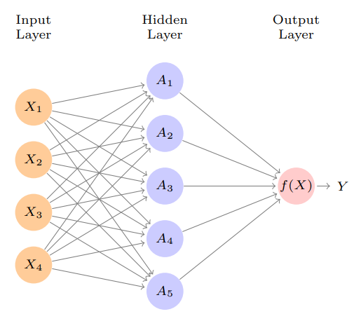
• $A_k=h_k(X)=g(w_{k0}+\sum^p_{j=1} w_{kj}X_j)$ are called the activations in the hidden layer
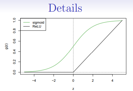
• $g(z)$ is called the activation function. Popular are the sigmoid and rectified linear, shown in figure
• Activation functions in hidden layers are typically nonlinear, otherwise the model collapses to a linear model
• So the activations are like derived features - nonlinear transformations of linear combinations of the features
• The model is fit by minimizing $\sum^n_{i=1}(y_i-f(x_i))^2$ (e.g. for regression)

Example : MNIST Digits

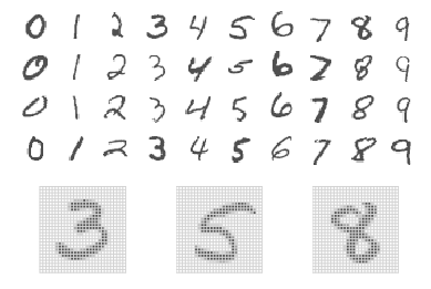
• Handwritten digits $28\times 28$ grayscale images $60K$ train, $10K$ test images
• Features are the $784$ pixel grayscale values $\in (0,255)$
• Labels are the digit class $0-9$

---

• Goal : build a classifier to predict the image class
• We build a two-layer network with $256$ units at first layer, $128$ units at second layer, and $10$ units at output layer
• Along with intercepts (called biases) there are $235,146$ parameters (referred to as weights)
  

---

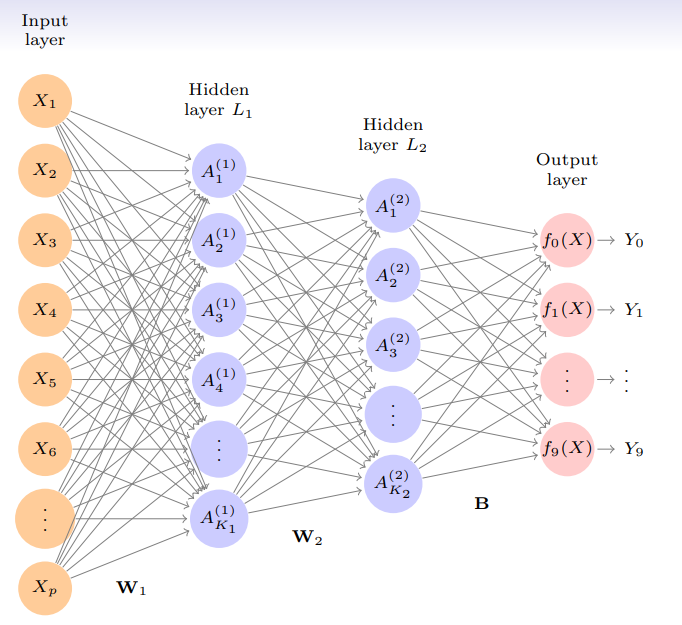
• Let $Z_m=\beta_{m0}+\sum^{K_2}_{l=1}\beta_{ml}A_l^{(2)},\;m=0,1,\dots,9$ be $10$ linear combinations of activations at second layer
• Output activation function encodes the softmax function
  $f_m(X)=\Pr(Y=m|X)=\frac{e^{Zm}}{\sum^9_{l=0}e^{Zl}}$
• We fit the model by minimizing the negative multinomial log-likelihood (or cross-entropy)
  $-\sum^n_{i=1}\sum^9_{m=0}y_{im}\log(f_m(x_i))$
• $y_{im}$ is $1$ if true class for observation $i$ is $m$, else $0$ - i.e. one-hot encoded

---

• Early success for neural networks in the 1990s
• With so many parameters, regularization is essential
• Some details of regularization and fitting will come later
• Very overworked problem - best reported rates are < $0.5\%$
• Human error rate is reported to be aroung $0.2\%$

Convolutional Neural Network - CNN

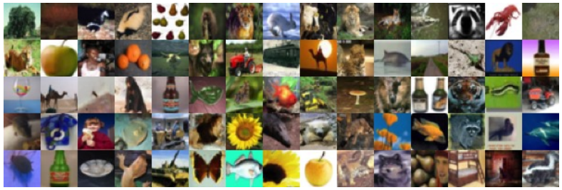
• Major success story for classifying images
• Shown are samples from CIFAR100 database
• $32\times 32$ color natural images, with $100$ classes
• $50K$ training images, $10K$ test images
• Each image is a three-dimensional array of feature map : $32\times32\times 3$ array of $8$-bit numbers
• The last dimension represents the three color channels for red, green and blue

---

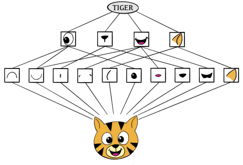
• The CNN builds up an image in a hierarchical fashion
• Edges and shapes are recognized and pieced together to form more complex shapes, eventually assembling the target image
• This hierarchical construction is achieved using convolution and pooling layers

Convolution Filter

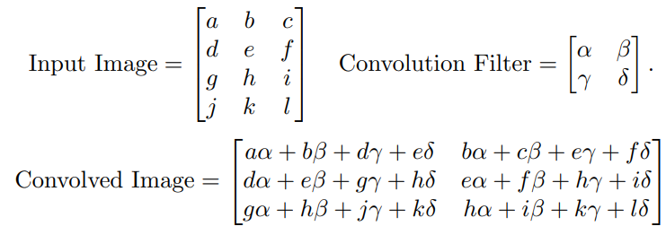
• The filter is itself an image, and represents a samll shape, edge etc.
• We slide it around the input image, scoring for matches
• The scoring is done via dot-products, illustrated above
• If the subimage of the input image is similar to the filter, the score is high, otherwise low
• The filters are learned during training
  

• The idea of convolution with a filter is to find common patterns that occur in differnet parts of the image
• The two filters shown here highlight vertical and horizontal stripes
• The result of the convolution is a new feature map
• Since images have three colors channels, the filter does as well : one filter per channel, and dot-products are summed
• The weights in the filters are learned by the network

Pooling

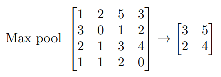
• Each non-overlapping $2\times 2$ block is replaced by its maximum
• This sharpens the feature identification
• Allows for locational invariance
• Reduces the dimension by a factor of $4$ - i.e. factor of $2$ in each dimension

Architecture of a CNN

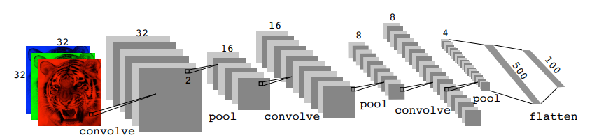
• Many convolve + pool layers
• Filters are typically small, e.g. each channel $3\times 3$
• Each filter creates a new channel in convolution layer
• As pooling reduces size, the number of filters/channels is typically increased
• Number of layers can be very large. E.g. resnet50 trained on imagenet 1000-class image data base has $50$ layers

Document Classification

Featurization : Bag-of-Words

• Documents have different lengths, and consist of sequences of words
• How do we create features $X$ to characterize a document?

---

• From a dictionary, identify the $10K$ most frequently occurring words
• Create a binary vector of length $p=10K$ for each document, and score a $1$ in every position that the corresponding word occurred
• With $n$ documents, we now have a $n\times p$ sparse feature matrix $X$
• We compare a lasso logistic regression model to a two-hidden-layer neural network on the next slide
• Bag-of-words are unigrams
• We can instead use bigrams ( occurrences of adjacent word pairs ), and in general m-grams

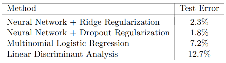
Lasso vs Neural Network

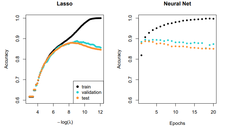
• Simpler lasso logistic regression model works as well as neural network in this case

Recurrent Neural Networks

• Often data arise as sequences :
  • Documents are sequences of words, and their relative positions have meaning
  • Time-series such as weather data or financial indices
  • Recorded speech or music
  • Handwriting, such as doctor's notes
• RNNs build models that take into account this sequential nature of the data, and build a memory of the past
  • The feature for each observation is a sequence of vectors $X=\{X_1,\dots,X_L\}$
  • The target $Y$ is often of the usual kind - e.g. a single variable such as Sentiment, or a one-hot vector for multiclass
  • However, $Y$ can also be a sequence, such as the same document in a differnet language

---

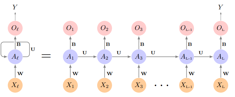
• The hidden layer is a sequence of vectors $A_l$, receiving as input $X_l$ as well as $A_{l-1}$
• $A_l$ produces an output $O_l$
• The same weights $W$, $U$ and $B$ are used at each step in the sequence - hence the term recurrent
• The $A_l$ sequence represents an evolving model for the response that is updated as each element $X_l$ is processed

---

• Suppose $X_l=(X_{l1},X_{l2},\dots,X_{lp})$ has $p$ components, and $A_l=(A_{l1},A_{l2},\dots,A_{lK})$ has $K$ components
• Then the computation at the $k$th components of hidden unit $A_l$ is
  $A_{lk}=g\left(w_{k0}+\sum^p_{j=1}w_{kj}X_{lj}+\sum^K_{s=1}u_{ks}A_{l-1,s}\right)\\[0.3cm] O_l=\beta_0+\sum^K_{k=1}\beta_kA_{lk}$
• Often we are concerned only with the prediction $O_L$ at the last unit
• For squared error loss, and $n$ sequence / response pairs, we would minimize
  $\sum_{i=1}^n (y_i - o_{iL})^2 = \sum_{i=1}^n \left( y_i - \left( \beta_0 + \sum_{k=1}^K \beta_k g \left( w_{k0} + \sum_{j=1}^p w_{kj} x_{iL_j} + \sum_{s=1}^K u_{ks} a_{i, L-1, s} \right) \right) \right)^2$

---

RNN and IMDB Reviews

• The document feature is a sequence of words $\{W_l\}^L_1$
• We typically truncate/pad the documents to the same number $L$ of words (we use $L=500$)
• Each word $W_l$ is represented as a one-hot encoded binary vector $X_l$ of length $10K$, with all zeros and a single one in the position for that word in the dictionary
• This results in an extremely sparse feature representation, and would not work well
• Instead we use a lower-dimensional pretrained work embedding matrix $E(m\times 10K)$
• This reduces the binary feature vector of length $10K$ to a real feature vector of dimension $m<10K$ (e.g. $m$ in the low hundreds)

Word Embedding

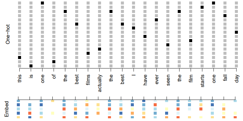
• Embeddings are pretrained on very large corpora of documents, using methods similar to principal components
• word2vec and GloVe are popular

---

• After a lot of work, the results are a disappointing $76\%$ accuracy
• We then fit a more exotic RNN than the one displayed - a LSTM with long and short term memory
• Here $A_l$ receives input from $A_{l-1}$ (short term memory) as well as from a version that reaches further back in time (long term memory)
• Now we get $87\%$ accuracy, slightly less than the $88\%$ achieved by glmnet
• These data have been used as a benchmark for new RNN architectures
• The best reported result found at the time of writing (2020) was aroung $95\%$
• We point to a leaderboard

Time Series Forecasting

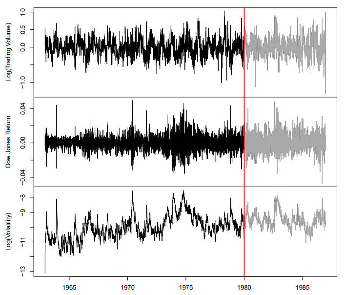
New-York Stock Exchange Data

• Shown in previous slide are three daily time series for the period $6,051$ trading days
  • Log trading volume : This is the fraction of all outstanding shares that are traded on that day, relative to a $100$-day moving average of past turnover, on the log scale
  • Dow Jones return : This is the difference between the log of the Dow Jones Industrial Index on consecutive trading days
  • Log volatility : This is based on the absolute values of daily price movements
• Goal : predict Log trading volume tomorrow, given it observed values up to today, as well as those of Dow Jones return and Log volatility

Autocorrelation

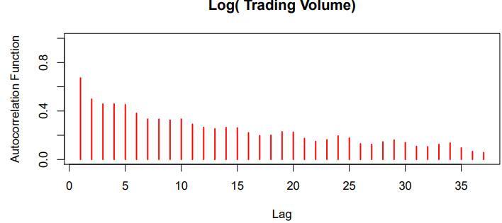
• The autocorrelation at lag $l$ is the correlation of all paris $(v_t,v_{t-l})$ that are $l$ trading days apart
• These sizable correlations give us confidence that past values will be helpful in predicting the future
• This is a curious prediction problem : the response $v_t$ is also a feature $v_{t-l}$

RNN Forecaster

• We only have one series of data
• How do we set up for an RNN
• We extract many short mini-series of input sequences $X=\{X_1,\dots,X_L\}$ with a predefined length $L$ known as the lag
  $X_1 = \begin{pmatrix} v_{t-L} \\ r_{t-L} \\ z_{t-L} \end{pmatrix}, \, X_2 = \begin{pmatrix} v_{t-L+1} \\ r_{t-L+1} \\ z_{t-L+1} \end{pmatrix}, \, \cdots, \, X_L = \begin{pmatrix} v_{t-1} \\ r_{t-1} \\ z_{t-1} \end{pmatrix}, \, \text{and } Y = v_t$
• Since $T=6,051$, with $L=5$ we can create $6,046$ such $(X,Y)$ pairs
• We use the first $4,281$ as training data, and the following $1,770$ as test data
• We fit an RNN with $12$ hidden units per lag step (i.e. per $A_l$)

---

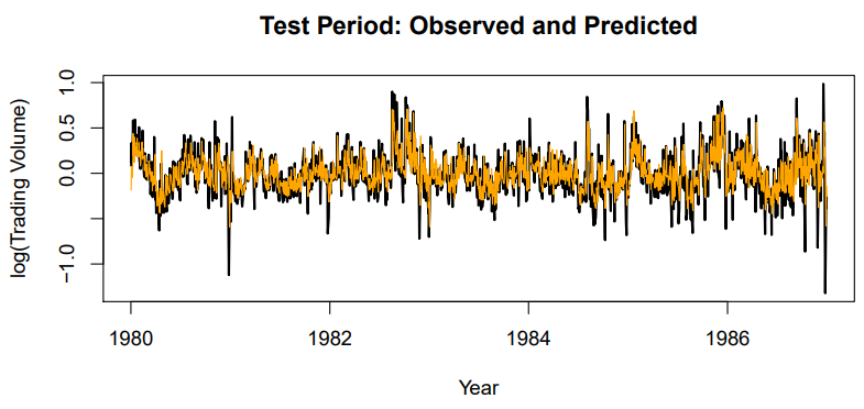
• Figure shows predictions and truth for test period
• $R^2=0.42$ for RNN
• $R^2=0.18$ for straw man - use yesterday's value of Log trading volume to predict that of today

Autoregression Forecaster

• The RNN forecaster is similar in structure to a traditional autoregression procedure
  $\mathbf{y} = \begin{bmatrix} v_{L+1} \\ v_{L+2} \\ v_{L+3} \\ \vdots \\ v_{T} \end{bmatrix} \quad \mathbf{M} = \begin{bmatrix} 1 & v_L & v_{L-1} & \cdots & v_1 \\ 1 & v_{L+1} & v_L & \cdots & v_2 \\ 1 & v_{L+2} & v_{L+1} & \cdots & v_3 \\ \vdots & \vdots & \vdots & \ddots & \vdots \\ 1 & v_{T-1} & v_{T-2} & \cdots & v_{T-L} \end{bmatrix}$
• Fit an OSL regression of $y$ on $M$, giving
  $\hat{v}_t = \hat{\beta}_0 + \hat{\beta}_1 v_{t-1} + \hat{\beta}_2 v_{t-2} + \cdots + \hat{\beta}_L v_{t-L}.$
• Known as an order-L autoregression model or $AR(L)$
• For the NYSE data we can include lagged version of DJ_return and log_volatility in matrix $M$, resulting in $3L+1$ columns

---

• $R^2=0.41$ for $AR(5)$ model ($16$ parameters)
• $R^2=0.42$ for RNN model ($205$ parameters)
• $R^2=0.42$ for $AR(5)$ model fit by neural network
• $R^2=0.46$ for all model if we include day_of_week of day being predicted

Non Convex Functions and Gradient Descent

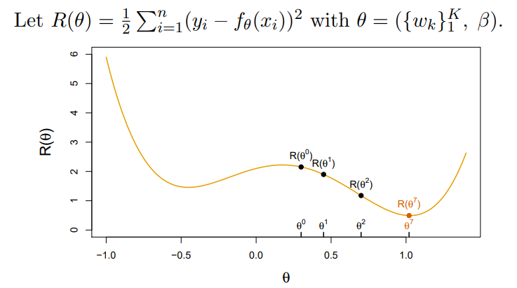
1. Start with a guess $\theta^0$ for all the parameters in $\theta$, and set $t=0$
2. Iterate until the objective $R(\theta)$ fails to decrease :
   2.1. Find a vector $\delta$ that reflects a small change in $\theta$, such that $\theta^{t+1}=\theta^t+\delta$ reduces the objective
   2.2. Set $t \leftarrow t+1$

---

• In this sample example we reached the global minimum
• If we had started a little to the left of $\theta^0$ we would have gone in the other direction, and ended up in a local minimum
• Although $\theta$ is multi-dimensional, we have depicted the process as one-dimensional
• It is much harder to identify whether one is in a local minimum in high dimensions
• How to find a direction $\delta$ that point downhill?
• We compute the gradient vector
  $\nabla R(\theta^t) = \left. \frac{\partial R(\theta)}{\partial \theta} \right|_{\theta = \theta^t}$
• i.e. the vector of partial derivatives at the current guess $\theta^t$
• The gradient points uphil, so our update is $\delta =-\rho\nabla R(\theta^t)$ or
  $\theta^{t+1} \leftarrow \theta^t - \rho \nabla R(\theta^t)$
  where $\rho$ is the learning rate (typically small, e.g. $\rho=0.001$)

Gradients and Backpropagation

is a sum, so gradient is sum of gradients

• For ease of notation, let $z_{ik}=w_{k0}+\sum^p_{j=1}w_{kj}x_{ij}$
• Backpropagation uses the chain rule for differentitaion
  $\frac{\partial R_i(\theta)}{\partial \beta_k} = \frac{\partial R_i(\theta)}{\partial f_\theta(x_i)} \cdot \frac{\partial f_\theta(x_i)}{\partial \beta_k} = - (y_i - f_\theta(x_i)) \cdot g(z_{ik}).\\[0.3cm] \frac{\partial R_i(\theta)}{\partial w_{kj}} = \frac{\partial R_i(\theta)}{\partial f_\theta(x_i)} \cdot \frac{\partial f_\theta(x_i)}{\partial g(z_{ik})} \cdot \frac{\partial g(z_{ik})}{\partial z_{ik}} \cdot \frac{\partial z_{ik}}{\partial w_{kj}} = - (y_i - f_\theta(x_i)) \cdot \beta_k \cdot g'(z_{ik}) \cdot x_{ij}.$

Tricks of the Trade

• Slow learning
  Gradient descent is slow, and a small learning rate $\rho$ slows it even further. With early stopping, this is a form of regularization
• Stochastic gradient descent
  Rather than compute the gradient using all the data, use a small minibatch drawn at random at each step
• An epoch is a count of iterations and amounts to the number of minibatch updates such that $n$ samples in total have been processed; i.e. $60K/128 \approx 469$ for MNIST
• Regularization
  Ridge and lasso regularization can be used to shrink the weights at each layer. Two other popular forms of regulariztion and dropout and augmentation

Droupout Learning

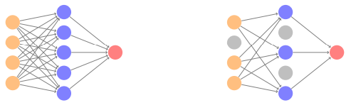
• At each SGD update, randomly remove units with probability $\phi$, and scale up the weights of those retained by $1/(1-\phi)$ to compensate
• In simple scenarios like linear regression, a version of this process can be shown to be equivalent to ridge regularization
• As in ridge, the other units stand in for those temporaily removed, and their weights are drawn closer together
• Similar to randomly omitting variables when growing trees in random forests

Ridge and Data Augmentation

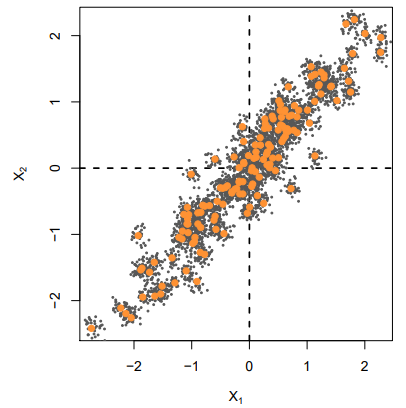
• Make many copies of each $(x_i,y_i)$ and add a small amount of Gaussian noise to the $x_i$ - a little cloud around each observation - but leave the copies of $y_i$ alone
• This makes the fit robust to small perturbations in $x_i$, and is equivalent to ridge regularization in an OLS setting

Double Descent

• With neural networks, it seems better to have too many hidden units than too few
• Likewise more hidden layers better than few
• Running stochastic gradients descent till zero training error often gives good out-of-sample error
• Increasing the number of units or layers and again training till zero error sometimes gives even better out-of-sample error
  
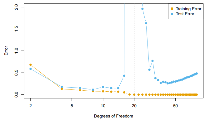
• When $d\leq 20$, model is OLS, and we see usual bias-variance trade-off
• When $d> 20$, we revert to minimum-norm
• As $d$ increases above $20$, $\sum^d_{j=1} \hat \beta_j^2$ decreases since it is easier to achieve zero error, and hence less wiggly solutions

• To achieve a zero-residual solution with $d=20$ is a real stretch
• Easier for larger $d$

---

• In a wide linear model ($p>n$) fit by least squares, SGD with a small step size leads to a minimum norm zero-residual solution
• Stochastic gradient flow - i.e. the entire path of SGD solutions - is somewhat similar to ridge path
• By analogy, deep and wide neural networks fit by SGD down to zero training error often give good solutions that generalize well
• In particular cases with high signal-to-noise ratio - e.g. image recognition - are less prone to overfitting; the zero-error solution is mostly signal

All Contents written based on GIST - Machine Learning & Deep Learning Lesson(Instructor : Prof. sun-dong. Kim)