Unsupervised Learning

• Most of this course focuses on supervised learning methods such as regression and classification
• In that setting we observe obth a set of features $X_1,X_2,\dots,X_p$ for each object, as well as a response or outcome variable $Y$
• The goal is then to predict $Y$ using $X_1,X_2,\dots,X_p$
• Here we instead focus on unsupervised learning, we where observe only the features $X_1,X_2,\dots,X_p$
• We are not interested in prediction, because we do not have an associated response variable $Y$

The Goals of Unsupervised Learning

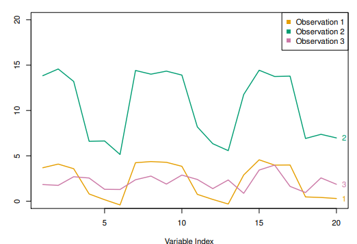
• The goal is to discover interesting things about the measurements :
  is there an informative way to visualize the data?
• Can we discover subgroups among the variables or among the observations?
• We discuss two methods
  • principal components analysis
    A tool used for data visulization or data pre-processing before supervised techniques are applied
  • clustering
    A broad class of methods for discovering unknown subgroups in data

Principal Components Analysis

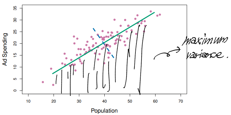
• PCA produces a low-dimensional representation of a dataset
• If finds a sequence of linear combinations of the variables that have maximal variance, and are mutually uncorrelated
• Apart from producing derived variables for use in supervised learning problems, PCA also serves as a tool for data visulization
• The first principal components of a set of features $X_1,X_2,\dots,X_p$ is the normalized linear combination of the features
  $Z_1=\phi_{11}X_1+\phi_{21}X_2+\dots+\phi_{p1}X_p$
  that has the largest variance. By normalized, we mean that $\sum^p_{j=1}\phi^2_{j1}=1$
• We refer to the elements $\phi_{11},\cdots,\phi_{p1}$ as the loadings of the first principal component; together, the loadings make up the principal component loading vector
  $\phi_1=\left(\phi_{11}\;\phi_{21}\;\dots\;\phi_{p1}\right)^T$
• We constrain the loadings so that their sum of squares is equal to one, since otherwise setting these elements to be arbitrarily large in absolute value could result in an arbitrarily large variance
  

Computation of Pricinpal Components

• Suppose we have a $n\times p$ data set $X$
• Since we are only interested in variance, we assume that each of the variables in $X$ has been centered to have mean zero (that is, the column means of $X$ are zero)
• We then look for the linear combination of the sample feature values of the form
  $z_{i1}=\phi_{11}x_{i1}+\phi_{21}x_{i2}+\cdots+\phi_{p1}x_{ip}$
  for $i=1,\dots,n$ that has largest sample variance, subject to the constraint that $\sum^p_{j=1}\phi^2_{j1}=1$
• Since each of the $x_{ij}$ has mean zero, then so does $z_{i1}$(for any value of $\phi_{j1})$
• Hence the sample variance of the $z_{i1}$ can be written as $\frac{1}{n}\sum^n_{i=1}z^2_{i1}$
• Plugging in (1) the first principal component loading vector solves the optimization problem
  $\text{maximize}_{\phi_{11}, \dots, \phi_{p1}} \frac{1}{n} \sum_{i=1}^n \left( \sum_{j=1}^p \phi_{j1} x_{ij} \right)^2 \text{subject to } \sum_{j=1}^p \phi_{j1}^2 = 1.$
• This problem can be solved via a singular-value decomposition of the matrix $X$, a standard technique in linear algebra
• We refer to $Z_1$ as the first principal component, with realized values $z_{11},\dots,z_{n1}$

Geometry of PCA

• The loading vector $\phi_1$ with elements $\phi_{11},\phi_{21},\dots,\phi_{p1}$ defines a direction in feature space along which the data vary the most
• If we project the $n$ data points $x_1,\dots,x_n$ onto this direction, the projected values are the principal component scores $z_{11},\dots,z_{n1}$ themselves

Further principal components

• The second principal component is the linear combination of $X_1,\dots,X_p$ that has maximal variance among all linear combinations that are uncorrelated with $Z_1$
• The second principal component scores $z_{12},z_{22},\dots,z_{n2}$ take the form
  $z_{i2}=\phi_{12}x_{i1}+\dots+\phi_{p2}x_{ip}$
  where $\phi_2$ is the second principal component loading vector, with elements $\phi_{12},\dots,\phi_{p2}$
• It turns out that constraining $Z_2$ to be uncorrelated with $Z_1$ is equivalent to constraining the direction $\phi_2$ to be orthogonal (perpendicular) to the direction $\phi_1$ And so on
• The principal component directions $\phi_1,\phi_2,\phi_3$ are the ordered sequence of right singular vectors of the matrix $X$, and the variance of the components are $\frac{1}{n}$ times the squares of the singular values
• There are at most $\min(n-1,p)$ principal components

  PCA should be performed after standardization

PCA find the hyperplane closest to the observations

• The first principal component loading vector has a very special property : it defines the line in $p$-dimensional space that is closest to the $n$ observations (using averae squared Euclidean distance as a measure of closeness)
• The notion of principal components as the dimensions that are closest to the $n$ observations extends beyond just the first principal component
• For instance, the first two principal components of a data set span the plan that is closest to the $n$ observations, in terms of average squared Euclidean distance

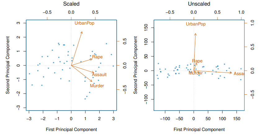
Scaling of the variables matters

• If the variables are in different units, scaling each to have standard deviation equal to one is recommended
• If they are in the same units, you might or might not scale the variables
  

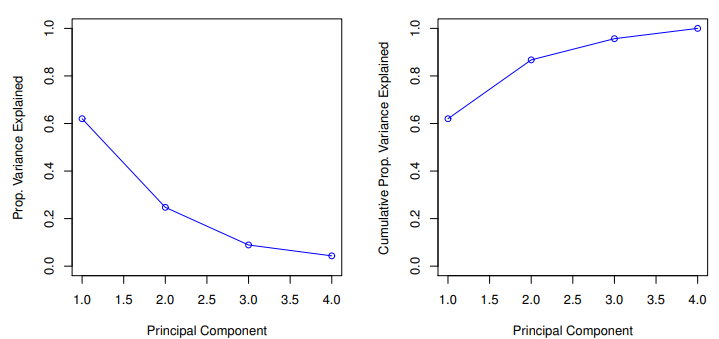
Proportion Variance Explained

• To understand the strength of each component, we are interested in knowing the proportion of variance explained (PVE) by each one
• The total variance present in a data set (assuming that the variables have been centered to have mean zero) is defined as
  $\sum^p_{j=1}\text{Var}(X_j)=\sum^p_{j=1}\frac{1}{n}\sum^n_{i=1}x_{ij}^2\\[0.2cm] n:\text{row},\quad j:\text{variables}$
  and the variance explained by the $m$th principal component is
  $\text{Var}(Z_m)=\frac{1}{n}\sum^n_{i=1}z^2_{im}$
• It can be shown that $\sum^p_{j=1}\text{Var}(X_j)=\sum^M_{m=1}\text{Var}(Z_m),\;\text{with }M=\min(n-1,p)$
• Therefore, the PVE of the $m$th principal component is given by the positive quantity between $0$ and $1$
  $\frac{\sum^n_{i=1}z^2_{im}}{\sum^p_{j=1}\sum^n_{i=1}x^2_{ij}}$
• The PVEs sum to one
• We sometimes display the cumlative PVEs
  

How many principal components should we use?

• If we use principal components as a summary of our data, how many components are sufficient?
  • No simple answer to this question, as cross-validation is not available for this purpose
    • Why not?
    • When could we use cross-validation to select the number of components?
  • the scree plot on the previous slide can be used as a guide : we look for an elbow

Matrix Completion via Principal Components

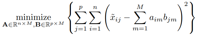
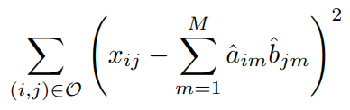
• We pose instead a modified version of the approximation criterion
  
  where $O$ is the set of all observed pairs of indices $(i,j)$ a subset of the possible $n\times p$ pairs
• Once we solve this problem :
  • we can estimate a missing observation $x_{ij}$ using $\hat x_{ij}=\sum^M_{m=1}\hat a_{im}\hat b_{jm}$, where $\hat a_{im}$ and $\hat b_{jm}$ are the $(i,m)$ and $(j,m)$ elements of the solution matrices $\hat A$ and $\hat B$
  • we can (approximately) recover the $M$ principal component scores and loadings, as if data were complete

Iterative Algorithm for Matirx Completion

1. Initialize : create a complete data matrix $\tilde X$ by filling in the missing value susing mean imputation
2. Repeat : step (a)-(c) until the objective in (c) fails to decreases
   • (a)
     by computing the principal components of $\tilde X$
   • (b) For each missing entry $(i,j)\not \in O,$ set $\tilde x_{ij} \leftarrow \sum^M_{m=1}\hat a_{im}\hat b_{im}$
   • (c) Compute the objective
     
3. Return the estimated missing entries $\tilde x_{ij},\;(i,j)\not \in O$

Clustering

K-means clustering

• Note that there is no ordering of the clusters, so that cluster coloring is arbitrary
• Let $C_1,\dots,C_K$ denotes sets containing the indices of the observations in each cluster
• These sets satisfy two properties
  1. $C_1\cup C_2 \cup \dots\cup C_K=\{1,\dots,n\}$. In other words, each observation belongs to at least one of the $K$ clusters
  2. $C_k \cap C_{k'}=\not 0$ for all $k\neq k'$
     In other words, the clusters are non-overlapping : no observation belongs to more than one cluster
  • For instnace, if the $i$th observation is in the $k$th cluster, then $i\in C_k$

---

• The idea begind $K$-means clustering is that a good clustering is one for which the within-cluster variation is as small as possible
• The within-cluster variation for cluster $C_k$ is a measure $\text{WCV}(C_k)$ of the amount by which the observations within a cluster differ from each other
• Hence we wnat to solve the problem
  $\text{minimize}_{C_1,\dots,C_K}\left\{\sum^K_{k=1}\text{WCV}(C_k)\right\}$
• In words, this formula says that we want to partition the observation into $K$ clusters such that the total within-cluster variation, summed over all $K$ clusters, is as small as possible

How to define within-cluster variation

• Typically we use Euclidean distance
  $\text{WCV}(C_k)=\frac{1}{|C_k|}\sum_{i,i'\in C_k}\sum^p_{j=1}(x_{ij}-x_{i'j})^2$
  where $|C_k|$ denotes the number of observations in the $k$th cluster
• Combining (2) and (3) gives the optimization problem that define $K$-means clustering
  $\text{minimize}_{C_1,\dots,C_K}\left\{\sum^K_{k=1}\frac{1}{|C_k|}\sum_{i,i'\in C_k}\sum^p_{j=1}(x_{ij}-x_{i'j})^2\right\}$

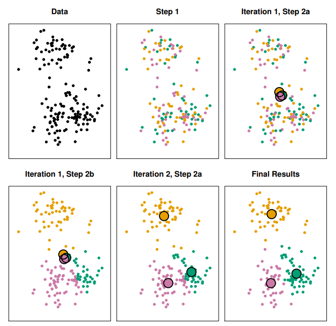
K-Means Clustering Algorithm

1. Randomly assign a number, from $1$ to $K$, to each of the observations. These serve as initial cluster assignments for the observations
2. Iterate until the cluster assignments stop changing
   2.1. For each of the $K$ clusters, compute the cluster centroid. The $k$th cluster centroid is the vector of the $p$ feature means for the observations in the $k$th cluster
   2.2. Assign each observation to the cluster whose centroid is closest (where closest is defined using Euclidean distance)

Properties of the Algorithm

• This algorithm is guaranteed to decrease the value of the objective (4) at each step
  $\frac{1}{|C_k|} \sum_{i,i' \in C_k} \sum_{j=1}^p (x_{ij} - x_{i'j})^2 = 2 \sum_{i \in C_k} \sum_{j=1}^p (x_{ij} - \bar{x}_{kj})^2, \\[0.2cm] \text{where } \bar{x}_{kj} = \frac{1}{|C_k|} \sum_{i \in C_k} x_{ij} \text{ is the mean for feature } j \text{ in cluster } C_k.$
• however it is not guaranteed to give the global minimum
  

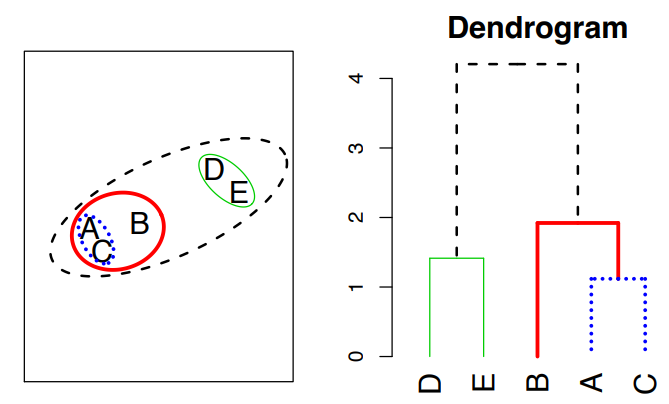
Hierarchical Clustering

• K-means requires us to pre-specify the number of clusters $K$
• We describe bottom-up or agglomerative clustering
• The approach in words :
  • Start with each point in its own cluster
  • Identify the closest two clusters and merge them
  • Repeat
  • Ends when all points are in a single cluster
    

Linkage

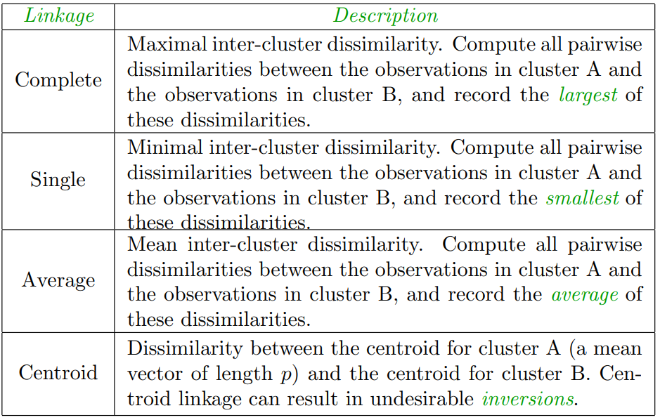
Choice of Dissimilarity Measure

• So far have used Euclidean distance
• An alternative is correlation-based distance which considers two observations to be similar if their features are highly correlated
• This is an unusual use of correlation, which is noramlly computed betwen variables; here it is computed between the observation profiles for each pair of observations
  

Practical issues

• Scaling of the variable matters
• Should the observations of features first be standardized in some way?
• For instance, maybe the variables should be centered to have mean zero and scaled to have standard deviation one
• In the case of hierarchical clustering,
  • What dissimilarity measure should be used?
  • What type of linkage should be used?
• How many clusters to choose? ( in both K-means or hierarchical clustering)

  Difficult problem

• No agreed-upon method
• Which features should we use to drive the clustering?

All Contents written based on GIST - Machine Learning & Deep Learning Lesson(Instructor : Prof. sun-dong. Kim)