추세

주식에서의 추세는 주가 또는 코인의 가격이 일정한 방향으로 일정 기간 계속 유지 되는 것

---

분류기

RandomForest를 기반으로 Bagging 수행

상승 : 1 / 하락 : 0

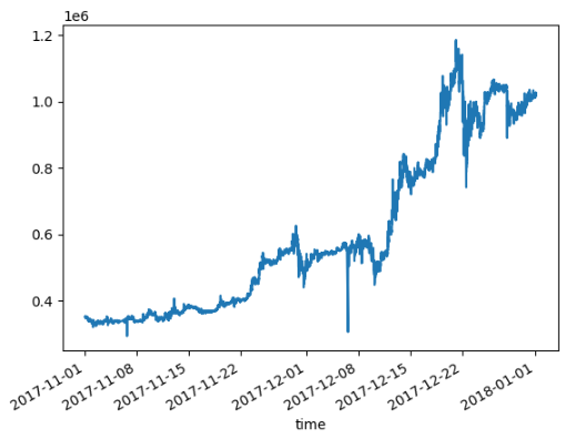
데이터 불러오기

import os
import pandas as pd
import numpy as np
import matplotlib.pyplot as plt
from tqdm import tqdm
import warnings
warnings.filterwarnings('ignore')

DATA_PATH = '/content/drive/MyDrive/DataSet/Aiffel/bitcoin/'
modify_data = pd.read_csv(os.path.join(DATA_PATH, 'sub_upbit_eth_min_tick.csv'), index_col=0, parse_dates=True)

modify_data.loc['2017-11-01':'2017-12-31','close'].plot()

---

Data Labeling

추세 라벨링 방법

1. Price Change Direction

2. Using Moving Average

3. Local Min-Max

4. Trend Scanning

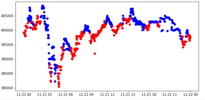
Price Change Direction

현재 종가와 과거의 종가 차이를 이용해 Label 진행

+ 면 상승 / - 면 하락으로 Labeling

window = 10
momentum_signal = np.sign(np.sign(modify_data['close'] - modify_data['close'].shift(window)) + 1)
s_momentum_signal = pd.Series(momentum_signal, index=modify_data.index)

sub_data = modify_data.loc['2017-11-21', 'close']
c_sig = s_momentum_signal.loc['2017-11-21']
c_sig['color'] = np.where(c_sig == 1, 'red', 'blue')

plt.figure(figsize=(10,5))
plt.scatter(sub_data.index, sub_data, c=c_sig['color'])

---

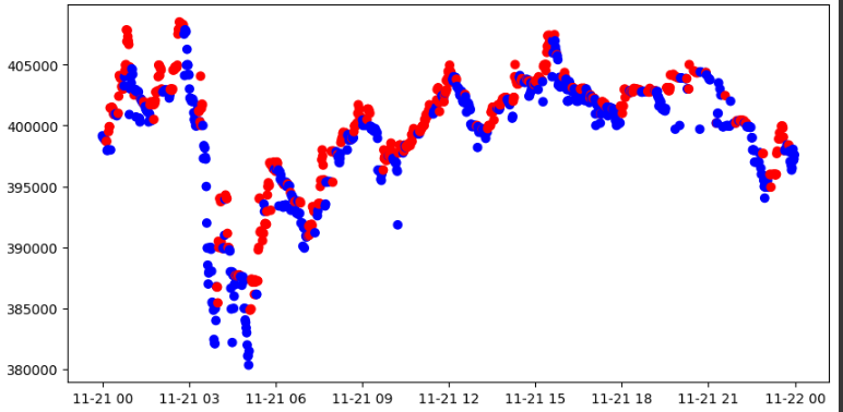
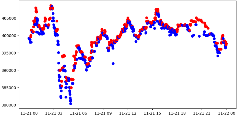
Using Moving Average

이동평균선을 구한 이후 현재 주가가 위, 아래 여부를 통해 Labeling

이동 평균을 몇일로 하느냐에 따라 Lag(지연)발생

위에 있으면 1 / 아래에 있으면 0

momentum_signal = np.sign(np.sign(modify_data['close'] - modify_data['close'].rolling(window).mean()) + 1)
s_momentum_signal = pd.Series(momentum_signal, index=modify_data.index)

sub_data = modify_data.loc['2017-11-21', 'close']
c_sig = s_momentum_signal.loc['2017-11-21']
c_sig['color'] = np.where(c_sig == 1, 'red', 'blue')

plt.figure(figsize=(10,5))
plt.scatter(sub_data.index, sub_data, c=c_sig['color'])

---

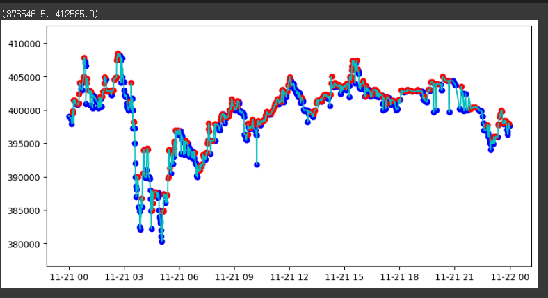
Local Min-Max

특정 구간에서의 최소, 최대값을 갱신하며 Label

ex) 하락 구간이어서 최소값이 계속 갱신되고 있다고 가정

1. 최대 값은 3000원이고 최소 값은 2800원

2. 현재 가격이 2750으로 낮아졌다면 최소값 변경

3. 다음 가격이 2800원으로 상승 할 경우 하락구간은 종료 되었다고 가정

4. 최소값인 2750을 최대값으로 설정 후 상승 구간 시작 으로 가정

현재 가격이 한번 상승했다고 바로 하락 구간을 종료하면 과도한 Labeling이 있을 수 있기에 변동이 적은 작업을 위해 Wait 계수 설정이 중요

# Local min / max 를 추출하기 위한 함수
def get_local_min_max(close, wait=3):
    min_value = close.iloc[0]
    max_value = close.iloc[0]
    n_cnt_min, n_cnt_max = 0, 0
    
    mins, maxes = [], []
    min_idxes, max_idxes = [], []
    b_min_update, b_max_update = False, False
    
    for idx, val in zip(close.index[1:], close.values[1:]):
        if val < min_value:
            min_value = val
            mins.append(min_value)
            min_idxes.append(idx)
            n_cnt_min = 0
            b_min_update = True
        if val > max_value:
            max_value = val
            maxes.append(max_value)
            max_idxes.append(idx)
            n_cnt_max = 0
            b_max_update = True
        
        if not b_max_update:
            b_min_update = False
            n_cnt_min += 1
            if n_cnt_min >= wait:
                max_value = min_value
                n_cnt_min = 0
    
        if not b_min_update:
            b_max_update = False
            n_cnt_max += 1
            if n_cnt_max >= wait:
                min_value = max_value
                n_cnt_max = 0
               
    return pd.DataFrame.from_dict({'min_time': min_idxes, 'local_min': mins}), pd.DataFrame.from_dict({'max_time': max_idxes, 'local_max': maxes})

mins, maxes = get_local_min_max(sub_data, wait=3)

fig, ax = plt.subplots(1, 1, figsize=(10, 5))
ax.plot(sub_data, 'c')
ax.scatter(mins.min_time, mins.local_min, c='blue')
ax.scatter(maxes.max_time, maxes.local_max, c='red')
ax.set_ylim([sub_data.min() * 0.99, sub_data.max()  * 1.01])

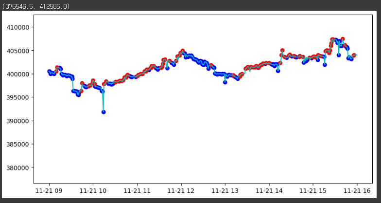
일부 데이터 사용

st_time, ed_time = '2017-11-21 09:00:00', '2017-11-21 16:00:00'

fig, ax = plt.subplots(1, 1, figsize=(10, 5))
ax.plot(sub_data.loc[st_time:ed_time], 'c')
ax.scatter(mins.set_index('min_time', drop=False).min_time.loc[st_time:ed_time], mins.set_index('min_time').local_min.loc[st_time:ed_time], c='blue')
ax.scatter(maxes.set_index('max_time', drop=False).max_time.loc[st_time:ed_time], maxes.set_index('max_time').local_max.loc[st_time:ed_time], c='red')
ax.set_ylim([sub_data.min() * 0.99, sub_data.max()  * 1.01])

---

Trend Scanning

t 시점에서 t + a까지 시점까지의 회귀식을 Fitting하여 𝛽(기울기) 값을 구한 이후 t-value를 계산

t-value가 양수면 t + a시점에는 상승할 가능성이 존재하며 음수일 경우 하락할 가능성이 존재

상승 예상 : 1 / 하락 예상 : 0

def t_val_lin_r(close):
    import statsmodels.api as sml
    
    # t-value from a linear trend
    x = np.ones((close.shape[0], 2))
    x[:, 1] = np.arange(close.shape[0])
    ols = sml.OLS(close, x).fit()
    return ols.tvalues[1]

look_forward_window = 60
min_sample_length = 5
step = 1
t1_array = []
t_values_array = []

molecule = modify_data['2017-11-01':'2017-11-30'].index
label = pd.DataFrame(index=molecule, columns=['t1', 't_val', 'bin'])
tmp_out = []

for ind in tqdm(molecule):
    subset = modify_data.loc[ind:, 'close'].iloc[:look_forward_window]  # 전방 탐색을 위한 샘플 추출
    if look_forward_window > subset.shape[0]:
        continue
    
    tmp_subset = pd.Series(index=subset.index[min_sample_length-1:subset.shape[0]-1])
    tval = []

    # 회귀분석을 통해 t 통계량값을 이용하여 추세 추정
    for forward_window in np.arange(min_sample_length, subset.shape[0]):
        df = subset.iloc[:forward_window]
        tval.append(t_val_lin_r(df.values))
    
    tmp_subset.loc[tmp_subset.index] = np.array(tval)
    idx_max = tmp_subset.replace([-np.inf, np.inf, np.nan], 0).abs().idxmax()
    tmp_t_val = tmp_subset[idx_max]
    tmp_out.append([tmp_subset.index[-1], tmp_t_val, np.sign(tmp_t_val)])

label.loc[molecule] = np.array(tmp_out)  # prevent leakage

label['t1'] = pd.to_datetime(label['t1'])
label['bin'] = pd.to_numeric(label['bin'], downcast='signed')