부제: Plotting Deer Sightings with Plotly
파일 설명
- UK Regional Population Data.csv
- 영국 인구 데이터
- Data resource - National Mammal Atlas Project.csv
- 영국에서 목격한 포유류
라이브러리 및 패키지 설치
import pandas as pd
import numpy as np
import matplotlib.pyplot as plt
import seaborn as sns
import warnings
import json

from urllib.request import urlopen

warnings.filterwarnings('ignore')

sns.set_theme() # 시각화의 테마(스타일)를 설정
데이터로드 및 데이터 살펴보기
df = pd.read_csv('/content/Data resource - National Mammal Atlas Project.csv')
df.head()
데이터 범위 설정
curr_df = df[df['Start date year'] >= 2000]
curr_df['Order'].value_counts()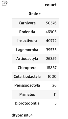
Plotly을 이용한 데이터 시각화
fig, ax = plt.subplots(1, 2, figsize = (14, 7))
years = [i for i in range(2000, 2024)]
big_palette = sns.color_palette("Spectral", n_colors = 24)
smol_palette = sns.color_palette("Spectral", n_colors = 6)
sns.countplot(curr_df, x = 'Start date year', ax = ax[0], palette = big_palette)
ax[0].set_title('Quantity of Observations Recorded Each Year')
ax[0].set_xlabel('Year')
ax[0].set_ylabel('Observations')
ax[0].set_xticklabels(years, rotation = 90)

temp = curr_df.groupby(['Start date year', 'Survey key']).count()['Common name'].reset_index()
surveys = [temp[temp['Start date year'] == i]['Survey key'].nunique() for i in years]
sns.lineplot(x = years, y = surveys, ax = ax[1])
ax[1].set_title('Quantity of Surveys Carried Out Each Year')
ax[1].set_xlabel('Year')
ax[1].set_ylabel('Surveys')

plt.show()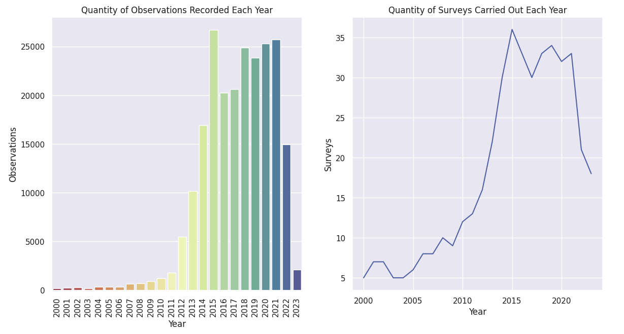
plot_df = curr_df.groupby(['Start date year', 'Order']).count()['Common name'].reset_index()
orders = plot_df['Order'].value_counts().index
obs = [plot_df[plot_df['Order'] == i] for i in orders]

#fill in the missing years for orders that have now observations
for n, i in enumerate(obs):
    for y in range(2000, 2024):
        if y not in list(i['Start date year']):
            new_row = pd.DataFrame({'Start date year': [y], 'Order': [orders[n]], 'Common name': [0]})
            i = pd.concat([i, new_row], ignore_index=True)
    i = i.sort_values('Start date year')
    obs[n] = list(i['Common name'])

#work out what proportion of observations were the given order in each year
for year in range(len(obs[0])):
    total = sum([i[year] for i in obs])
    for order in range(len(obs)):
        obs[order][year] =  obs[order][year]/total


obs.insert(0, [i for i in range(2000, 2024)])
sns.set_palette(smol_palette)
fig, ax = plt.subplots(figsize = (16, 8))
plt.stackplot(*obs, labels = orders)
plt.legend(loc = 'center left', bbox_to_anchor = (1, 0.5))
ax.set_title('Proportion of Observations That are Given Order of Animal')
ax.set_xlabel('Year')
ax.set_ylabel('Proportion')
ax.set_xlim(2000, 2023)
ax.set_ylim(0, 1)
plt.show()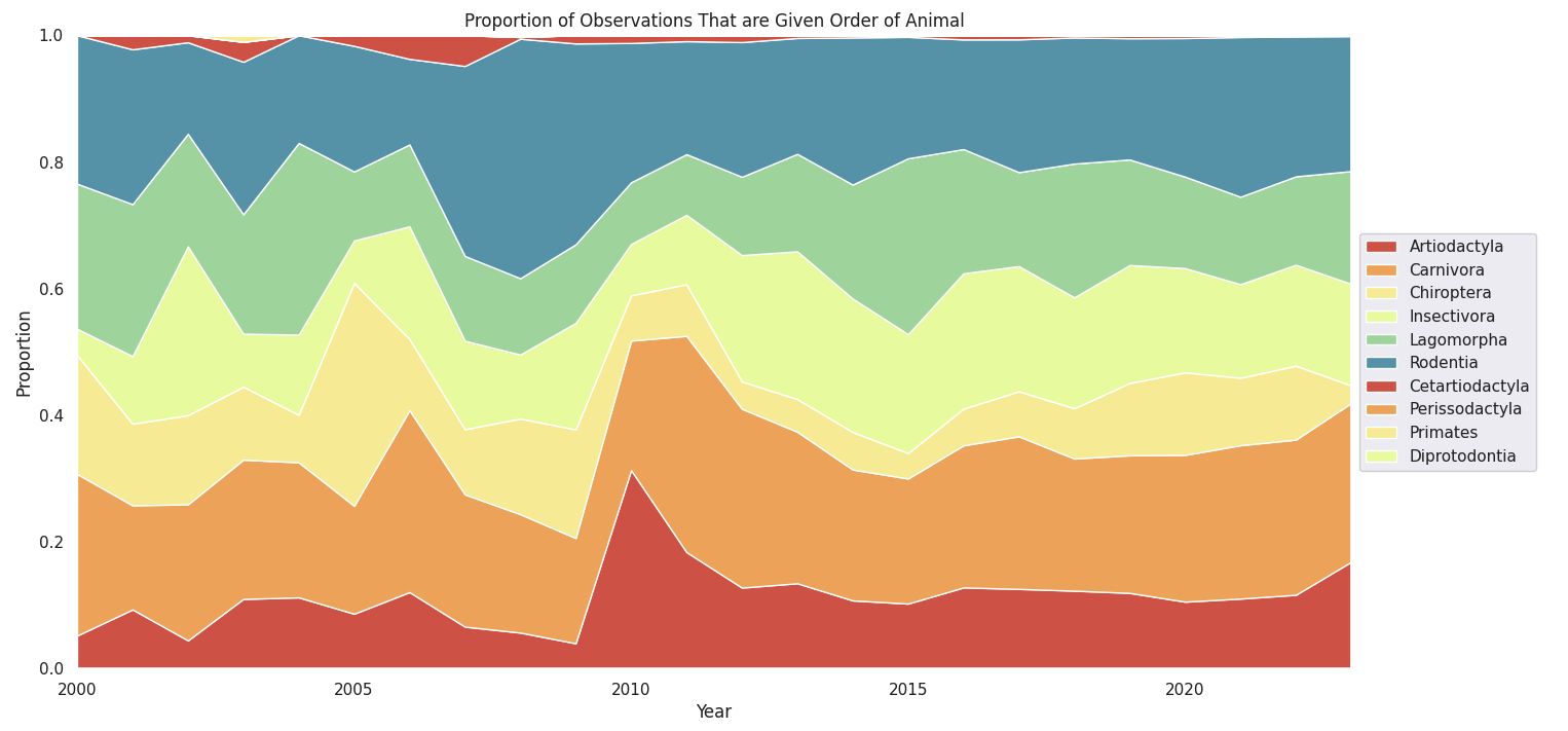
분석
# 사슴 종류
deer_df = curr_df[curr_df['Order'] == 'Artiodactyla']
deer_df['Common name'].value_counts()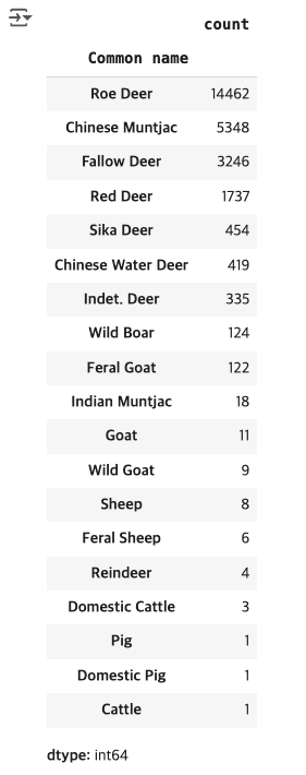
roe_df = deer_df[deer_df['Common name'] == 'Fallow Deer']
roe_df.head()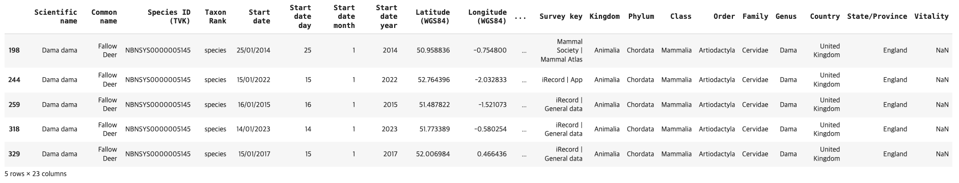
fig, ax = plt.subplots(1, 2, figsize = (14, 7))
big_palette = sns.color_palette("Spectral", n_colors = 24)
sns.countplot(roe_df, x = 'Start date year', ax = ax[0], palette = big_palette)
years = roe_df['Start date year'].value_counts().index.sort_values()
ax[0].set_xticklabels(years, rotation = 90)
ax[0].set_title('Quantity of Observations Recorded Each Year')
ax[0].set_xlabel('Year')
ax[0].set_ylabel('Observations')

temp = roe_df.groupby(['Start date year', 'Survey key']).count()['Common name'].reset_index()
surveys = [temp[temp['Start date year'] == i]['Survey key'].nunique() for i in years]
sns.lineplot(x = years, y = surveys, ax = ax[1])
ax[1].set_title('Quantity of Surveys Carried Out Each Year')
ax[1].set_xlabel('Year')
ax[1].set_ylabel('Surveys')

plt.show()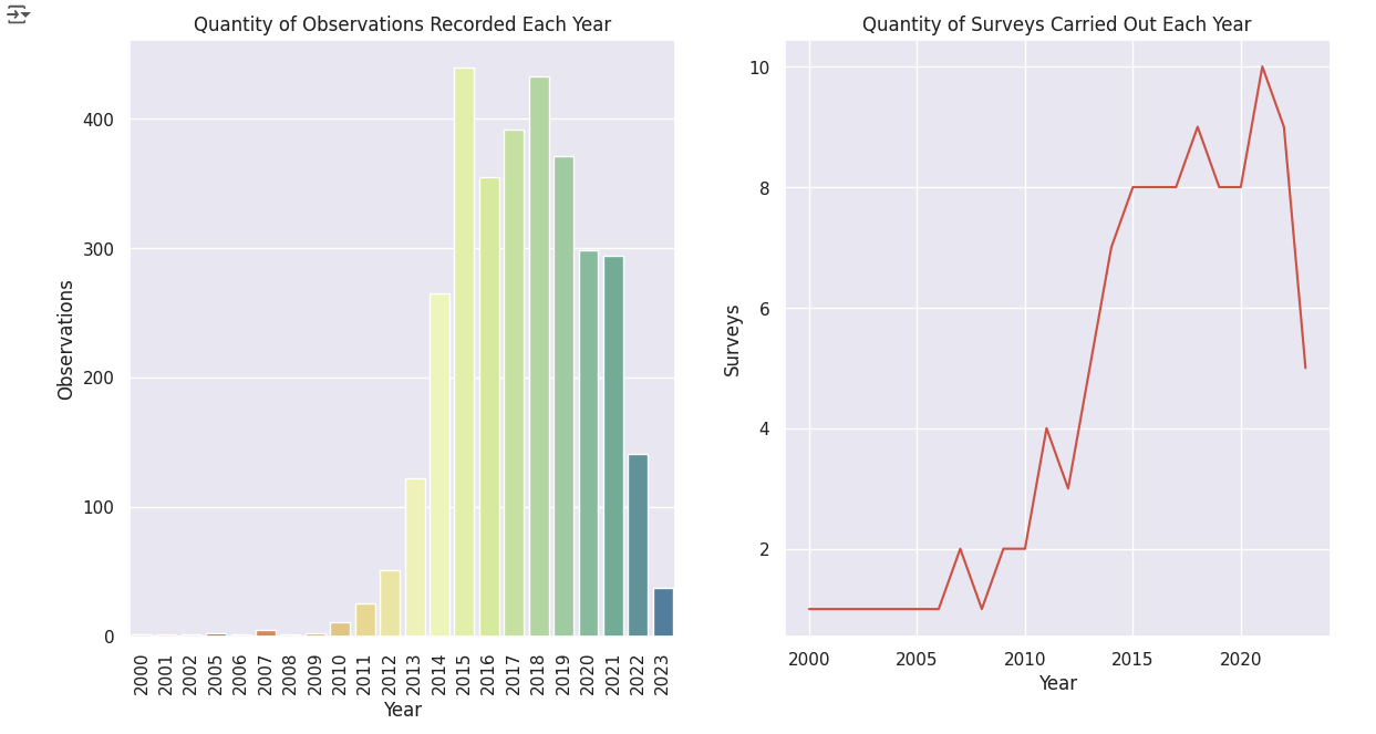
# JSON 파일과 CSV 파일을 불러와 데이터를 병합
import json

with open('/content/Local_Authority_Districts_(December_2021)_GB_BFC.json', 'r') as response:
    Local_authorities = json.load(response)


la_data = []
for i in range(len(Local_authorities["features"])):
    la = Local_authorities["features"][i]['properties']['LAD21NM']
    Local_authorities["features"][i]['id'] = la
    la_data.append([la,i])


pop_df = pd.read_csv('/content/UK Regional Population Data.csv') # Replace with your CSV file path
df = pd.DataFrame(la_data)
df.columns = ['LA','Val']
pops = []
for i in df['LA']:
    pops.append(pop_df[pop_df['Name'] == i]['Estimated Population mid-2021'].iloc[0])
df['Val'] = pops
roe2021_df = roe_df[roe_df['Start date year'] == 2021]
roe2021_df.head()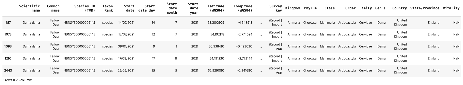
# 영국에 사슴 분포도
import plotly.express as px

fig = px.scatter_mapbox(roe2021_df,
                     lat = 'Latitude (WGS84)',
                     lon = 'Longitude (WGS84)',
                     mapbox_style="carto-positron",
                     title="Automatic Labels Based on Data Frame Column Names")

fig_px = px.choropleth_mapbox(df,
                              geojson=Local_authorities,
                              locations='LA',
                              color='Val',
                              featureidkey="properties.LAD21NM",
                              mapbox_style="carto-positron",
                              color_continuous_scale = px.colors.sequential.Greens,
                              labels={'val':'value'},
                              zoom = 4.5,
                              center={"lat": 55.09621, "lon": -4.0286298},
                              title="Automatic Labels Based on Data Frame Column Names")


fig_px.add_trace(
    fig.data[0]
)

fig_px.update_layout(margin={"r":0,"t":0,"l":0,"b":0})
fig_px.show()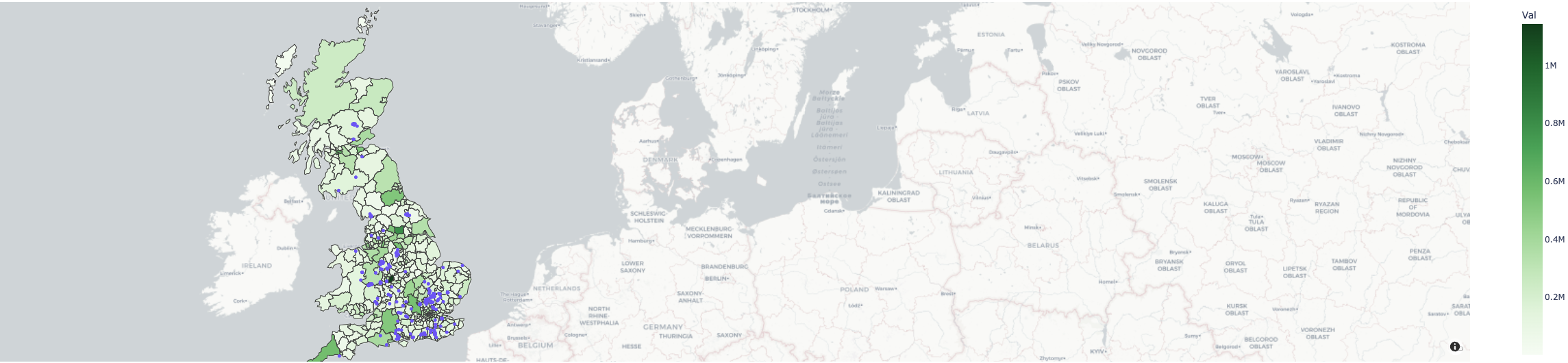
결론
Plotly을 이용한 데이터 분석, 영국의 야생동물 데이터와 영국인구 데이터를 이용하여 영국의 사슴종류와 출현시기, 출현횟수등을 분석하여 영국의 사슴분석도를 나타냄으로써 Plotly의 사용법과 효과에 대해 이해함

개발자를 위한 첫시작