지금까지 딥러닝 모델은 단순히 사용자가 부여한 아이템의 평점만을 이용하여 추천을 했지만, 현업에서는 user_id와 movie_id만 있는 상황이 아니다. 그 외에도 다양한 변수들이 있기 때문에 그 다양한 변수들을 활용해서 모델을 구성해보려 한다.
만약 직업에 따라서 영화의 평가 경향이 존재한다면, 직업이라는 요소를 추가하여 모델을 구성할 수 있을 것이다. 그러므로 그러한 다양한 요소를 추가할 수 있는 방법론에 대한 것이다.
직업이라는 범주형 변수를 user_id와 함께 받아온 후, 종류에 따라 인코딩한다.
one-hot representation과 embedding layer를 연결한 새로운 행렬을 만들고, Flatten() 한 뒤, P, Q 행렬, 사용자 bias, 아이템 bias와 다함께 concatenate() 해준다.
import pandas as pd
from sklearn.model_selection import train_test_split

# 필요한 tensorflow 모듈들을 가져온다.
import tensorflow as tf
from tensorflow.keras import layers
from tensorflow.keras.models import Model
from tensorflow.keras.layers import Input, Embedding, Dot, Add, Flatten
# layer 구성에 필요한 라이브러리 불러오기
from tensorflow.keras.layers import Dense, Concatenate, Activation
from tensorflow.keras.regularizers import l2
from tensorflow.keras.optimizers import SGD, Adamax

# 데이터 준비
r_cols = ['user_id', 'movie_id', 'rating', 'timestamp']
ratings = pd.read_csv('drive/MyDrive/RecoSys/data/u.data',
                      names = r_cols,
                      sep = '\t',
                      encoding = 'latin-1')

ratings_train, ratings_test = train_test_split(ratings,
                                               test_size = 0.2,
                                               shuffle = True,
                                               random_state = 2024)

# 직업이라는 변수를 추가하고 싶기 때문에 u.user 데이터 받아온다.
u_cols = ['user_id', 'age', 'sex', 'occupation', 'zip_code']
users = pd.read_csv('drive/MyDrive/RecoSys/data/u.user',
                    names = u_cols,
                    sep = '|',
                    encoding = 'latin-1')

 # 사용자 ID와 직업만 남긴다.
users = users[['user_id', 'occupation']]

occupation = {} #직업을 딕셔너리 형태로 바꿀 것이다. 문자열로 들어가 있는 값을 수치형 데이터로 바꾸기 위한 작업
def convert_occ(x):
  if x in occupation:
    return occupation[x]
  else:
    occupation[x] = len(occupation) #occupation딕셔너리에는 직업이 순차적으로 값을 받게 된다.
    return occupation[x]

users['occupation'] = users['occupation'].apply(convert_occ) #직업 범주형 변수 인코딩 완료

L = len(occupation) #여기서는 bias term이 없으니까 +1 하지 않는다.
###############################
train_occ = pd.merge(ratings_train, users, on = 'user_id')['occupation']
test_occ = pd.merge(ratings_test, users, on = 'user_id')['occupation']

def RMSE(y_true, y_pred):
  return tf.sqrt(tf.reduce_mean(tf.square(y_true - y_pred)))

K = 200

mu = ratings_train.mean()

M = ratings['user_id'].max() + 1
N = ratings['movie_id'].max() + 1

user = Input(shape = (1,))
item = Input(shape = (1,))

P_embedding = Embedding(M, K, embeddings_regularizer = l2())(user)
Q_embedding = Embedding(N, K, embeddings_regularizer = l2())(item)

user_bias = Embedding(M, 1, embeddings_regularizer = l2())(user)
item_bias = Embedding(N, 1, embeddings_regularizer = l2())(item)

P_embedding = Flatten()(P_embedding)
Q_embedding = Flatten()(Q_embedding)

user_bias = Flatten()(user_bias)
item_bias = Flatten()(item_bias)

occ = Input(shape = (1,))
OCC_embedding = Embedding(L, 3, embeddings_regularizer = l2())(occ) #occupation 딕셔너리의 길이이므로 전체 직업의 종류 개수 L, latent vector 3
OCC_layer = Flatten()(OCC_embedding)

R = Concatenate()([P_embedding, Q_embedding, user_bias, item_bias, OCC_layer])

R = Dense(2048)(R)
R = Activation('linear')(R)
R = Dense(256)(R)
R = Activation('linear')(R)
R = Dense(1)(R)

model = Model(inputs = [user, item, occ], outputs = R)

model.compile(
    loss = RMSE,
    optimizer = SGD(),
    metrics = [RMSE]
)

model.summary()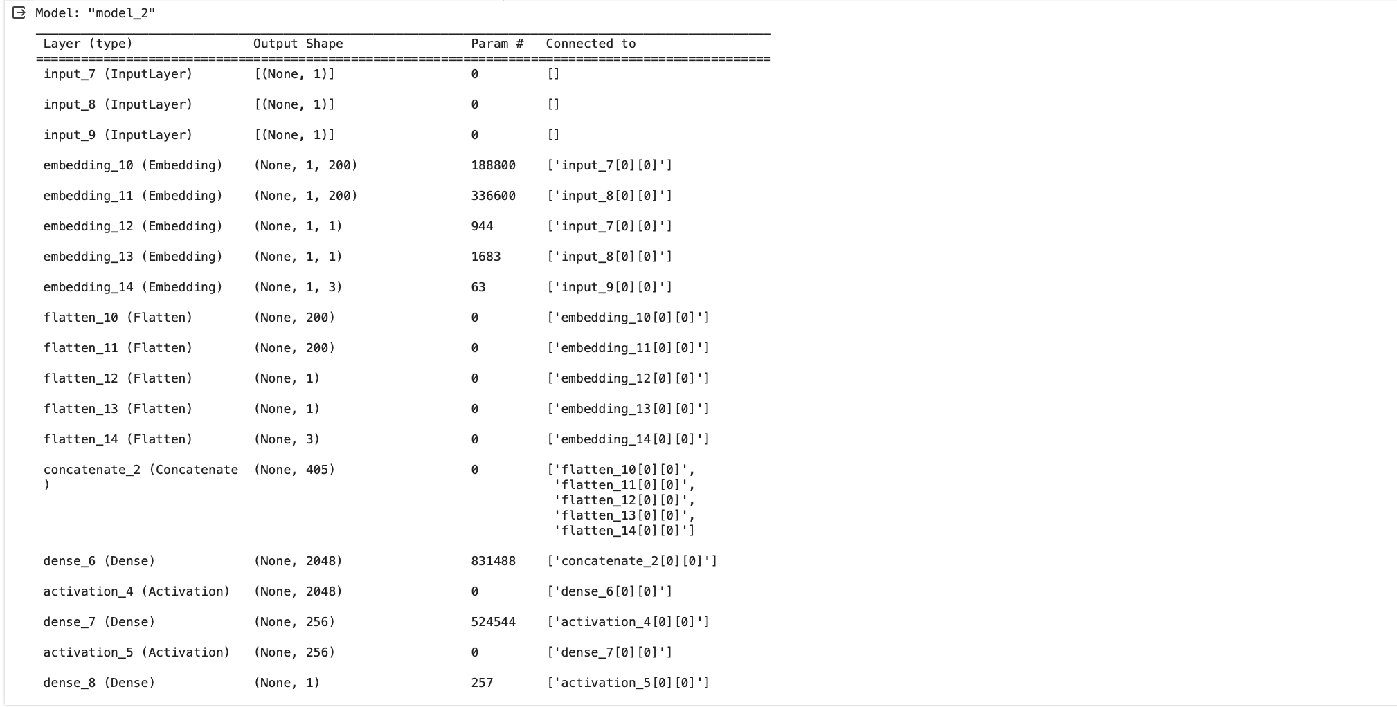
사용자 임베딩(P 행렬), 아이템 임베딩(Q 행렬), 사용자 bias 아이템 bias, 직업 임베딩을 모두 concatenate()했기 때문에 (200 + 200 + 1 + 1 + 3 = 405) 405 크기인 것을 알 수 있다.
여기서 3은 직업 임베딩의 latent vector를 3으로 지정했기 때문이다.
# Model Fitting
train_user_ids = ratings_train['user_id'].values
train_movie_ids = ratings_train['movie_id'].values
train_ratings = ratings_train['rating'].values
train_occs = train_occ.values

test_user_ids = ratings_test['user_id'].values
test_movie_ids = ratings_test['movie_id'].values
test_ratings = ratings_test['rating'].values
test_occs = test_occ.values

result = model.fit(
    x = [train_user_ids, train_movie_ids, train_occs],
    y = train_ratings - mu,
    epochs = 65,
    batch_size = 512,
    validation_data = (
        [test_user_ids, test_movie_ids, test_occs],
        test_ratings - mu
    )
)
학습이 잘 되었는지 그래프로 표현
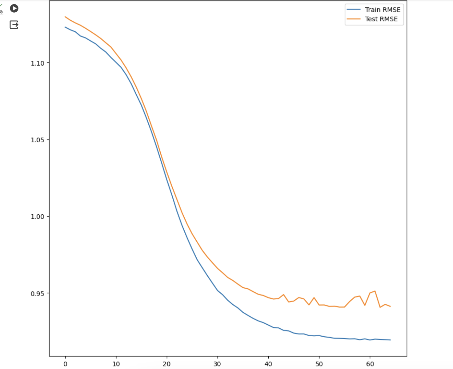
직업을 고려하지 않은 앞에서의 신경망과 비교해서 RMSE가 그렇게 눈에 띄게 향상되지는 않았다.
사용자의 평가 패턴과 상관이 있는 변수를 추가한다면 모델 성능을 향상 시킬 수 있을 것이다.

data analysis, data science