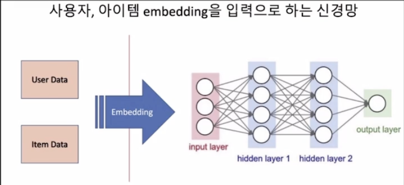
MF를 신경망으로 구성할 때, 사용자 데이터와 아이템 데이터를 embedding해서 입력으로 사용했다.
그 점은 똑같게 적용시킬 것이지만, 이제는 MF를 신경망으로 구성한 것에서 hidden layer가 추가된다.
hidden layer 은닉층을 사용해 만든 추천 시스템 구조
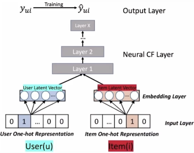
사용자 잠재요인과 아이템 잠재요인(embedding layer)을 합쳐서 첫번째 layer층을 만드는데,
가장 단순한 방법인 concatenate(단순 결합)를 사용한다.
import pandas as pd
from sklearn.model_selection import train_test_split

# 필요한 tensorflow 모듈들을 가져온다.
import tensorflow as tf
from tensorflow.keras import layers
from tensorflow.keras.models import Model
from tensorflow.keras.layers import Input, Embedding, Dot, Add, Flatten
# layer 구성에 필요한 라이브러리 불러오기
from tensorflow.keras.layers import Dense, Concatenate, Activation
from tensorflow.keras.regularizers import l2
from tensorflow.keras.optimizers import SGD, Adamax

# 데이터 준비
r_cols = ['user_id', 'movie_id', 'rating', 'timestamp']
ratings = pd.read_csv('drive/MyDrive/RecoSys/data/u.data',
                      names = r_cols,
                      sep = '\t',
                      encoding = 'latin-1')

ratings_train, ratings_test = train_test_split(ratings,
                                               test_size = 0.2,
                                               shuffle = True,
                                               random_state = 2024)

def RMSE(y_true, y_pred):
  return tf.sqrt(tf.reduce_mean(y_true, y_pred))

# Variable 초기화
# y_true, y_pred는 신경망에서 실제값, 예측값을 나타내는 Tensorflow/Keras 표준 변수이다.
K = 200
mu = ratings_train['rating'].mean()

M = ratings['user_id'].max() + 1 #movie lens데이터는 정리가 잘 되어있어서 max로 한 것.
N = ratings['movie_id'].max() + 1 #다른 데이터라면, unique()가 맞음
Keras Model
# 아래 부분은 앞에서와 동일하게 사용자와 아이템 데이터를 embedding을 통해
# 각각 K개의 노드를 갖는 layer로 변환하고
# 사용자 bias와 아이템 bias를 1개의 노드를 갖는 layer로 변환한다.
user = Input(shape = (1,))
item = Input(shape = (1,))

P_embedding = Embedding(M, K, embeddings_regularizer = l2())(user)
Q_embedding = Embedding(N, K, embeddings_regularizer = l2())(item)

user_bias = Embedding(M, 1, embeddings_regularizer = l2())(user)
item_bias = Embedding(N, 1, embeddings_regularizer = l2())(item)

P_embedding = Flatten()(P_embedding)
Q_embedding = Flatten()(Q_embedding)

user_bias = Flatten()(user_bias)
item_bias = Flatten()(item_bias)

R = Concatenate()([P_embedding, Q_embedding, user_bias, item_bias])

R = Dense(2048)(R) #노드가 2048개인 하나의 layer를 만들어준다. concatenate 된 R과 연결
R = Activation('linear')(R) #

R = Dense(256)(R)
R = Activation('linear')(R)

R = Dense(1)(R) #출력 노드 설정

model = Model(inputs = [user, item], outputs = R)

model.compile(
    loss = RMSE,
    optimizer = SGD(),
    metrics = [RMSE]
)

model.summary()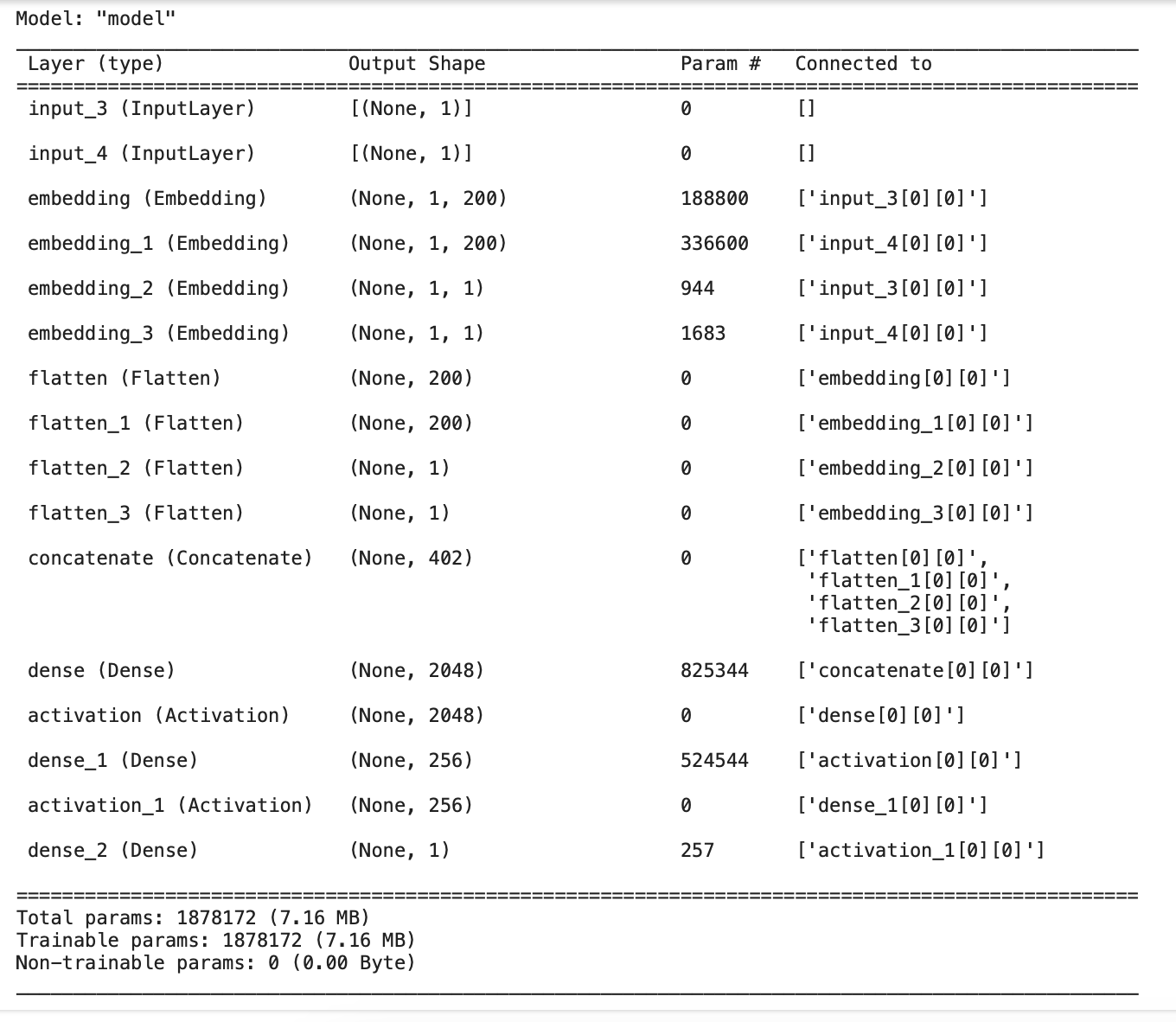
각각의 P_embedding, Q_embedding, user_bias, item_bias 모두 flatten 해주는 이유는 concatenate하기 위해서이다.
concatenate의 param수 = 402 (200 + 200 + 1 + 1)
Model Fitting
# Model Fitting
# 모델 입력에 필요한 데이터 정리
train_user_ids = ratings_train['user_id'].values
train_movie_ids = ratings_train['movie_id'].values
train_ratings = ratings_train['rating'].values

test_user_ids = ratings_test['user_id'].values
test_movie_ids = ratings_test['movie_id'].values
test_ratings = ratings_test['rating'].values

result = model.fit(
    x = [train_user_ids, train_movie_ids],
    y = train_ratings - mu,
    epochs = 65,
    batch_size = 512, #비효율적인 리소스 사용으로 인해 batch_size로 데이터를 나누어 학습을 진행한다.
    validation_data = (
        [test_user_ids, test_movie_ids],
        test_ratings - mu
    )
)
그래프를 통해 학습 결과 확인
import matplotlib.pyplot as plt

plt.figure(figsize = (10, 10))
plt.plot(result.history['RMSE'], labels = "Train RMSE")
plt.plot(result.history['val_RMSE'], label = "Test RMSE")
plt.legend()
plt.show()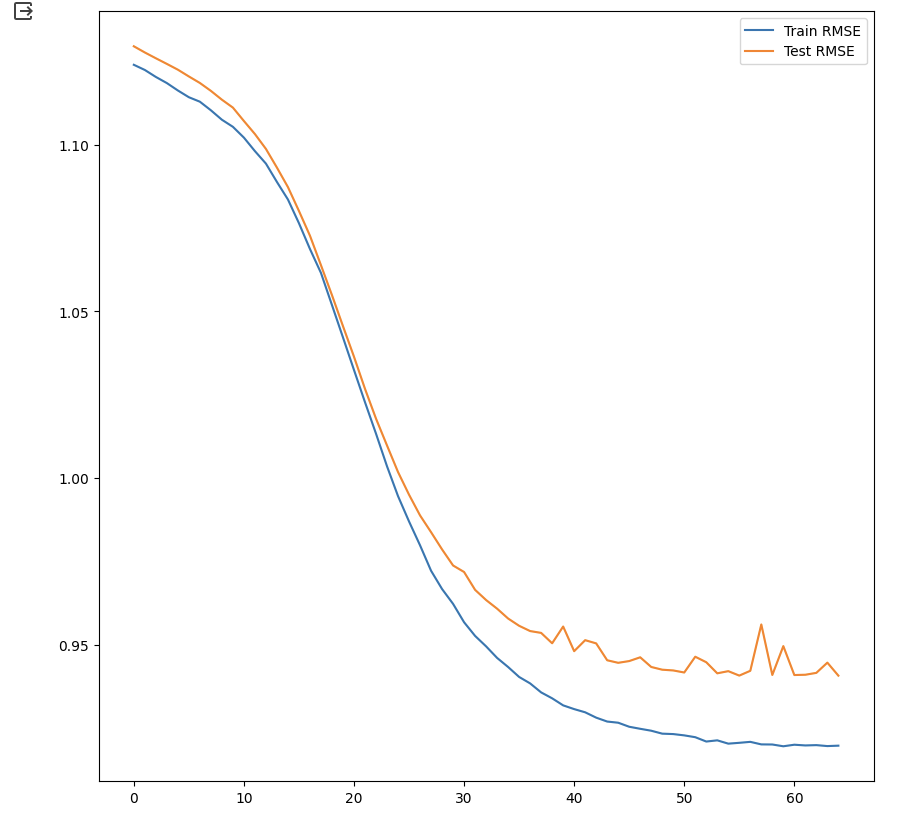
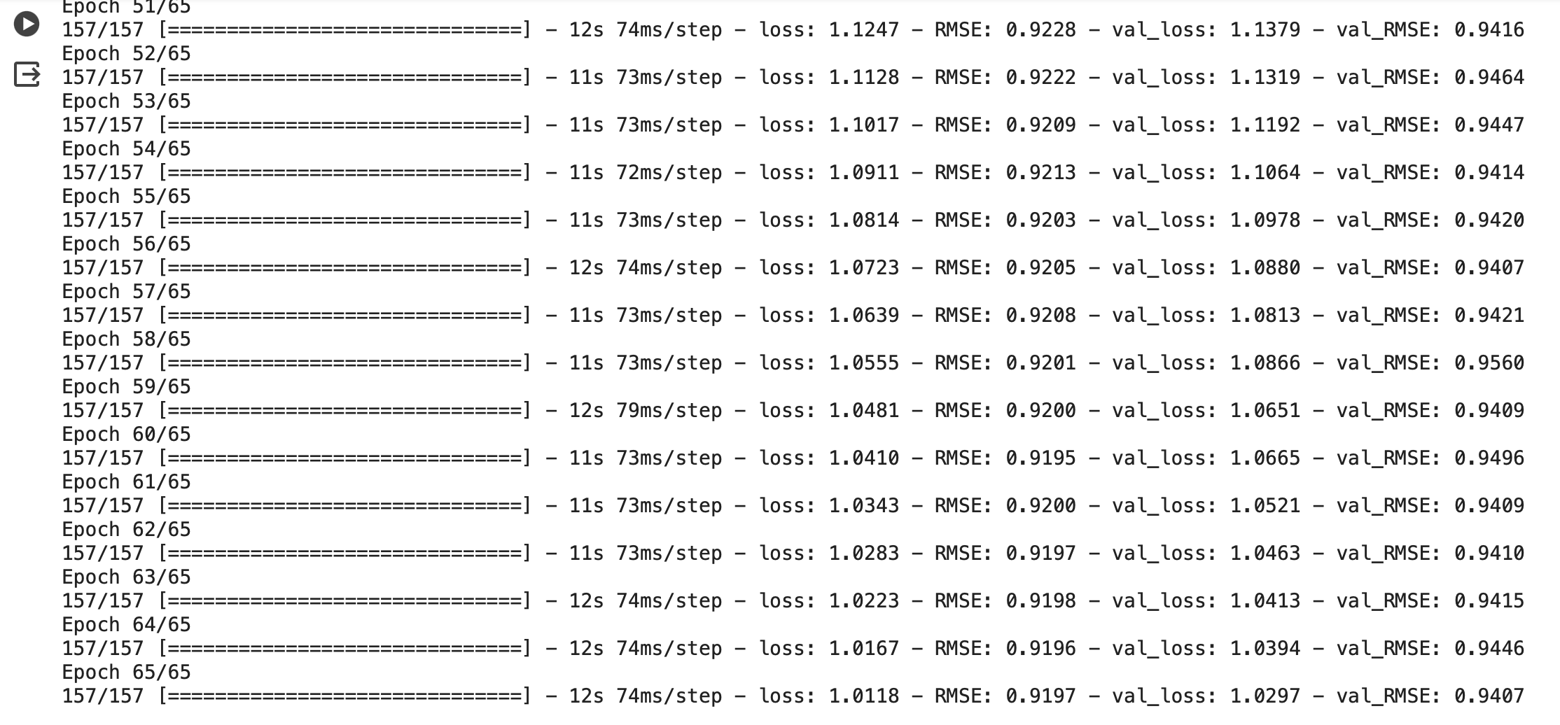
뒤쪽의 epoch에서는 약간의 Fluctuation이 나타나는 것을 볼 수 있다.
Fluctuation은 보통 과적합 때문에 일어나는 현상이라고 보는데, 그럼에도 불구하고, MF만 신경망으로 구현한 것보다는 성능이 많이 개선된 것을 볼 수 있다.
그렇다고 해서 항상 딥러닝을 사용한 것이 가장 성능이 좋은 것은 아니다.
데이터에 따라 달라지는데, 가령 연속값으로 평가값 데이터가 많이 풍부한 경우에는 MF의 성능이 상당히 좋은데,
만약 데이터가 binary 하거나 좀 숫자가 아닌 경우 혹은 좀 희박한 데이터(sparse data)를 가진 경우에는 MF보다는 딥러닝이 성능이 좋다.

data analysis, data science