Boosting Zero-shot Learning via Contrastive Optimization of Attribute Representations 제3-2부 method

4) Inference: At testing, the input class-semantics for seen class are replaced by the corresponding semantics of unseen classes (for ZSL) or of all classes (for GZSL) to embed new sets of class prototypes.
embede 포함하다. 내장되다.
4) 추론: 테스트에서 보이는 클래스에 대한 입력 클래스 시맨틱은 새로운 클래스 프로토타입 세트를 내장하기 위해 보이지 않는 클래스(ZSL) 또는 모든 클래스(GZSL)의 해당 시맨틱으로 대체된다.

We compute the cosine similarities from the class-level feature of a test image to embedded class prototypes to decide the class label of the image.
우리는 이미지의 클래스 레이블을 결정하기 위해 테스트 이미지의 클래스 레벨 기능에서 임베디드 클래스 프로토타입까지 코사인 유사성을 계산한다.

C. Class representation learning

Given the class semantics in CS, each $cs_i$ is in the form of a K-dimensional vector indicating the presence/absence of the K attributes in this class.
CS의 클래스 의미론이 주어지면 각 $cs_i$는이 클래스에서 K 속성의 존재 / 부재를 나타내는 K 차원 벡터의 형태입니다.
The digits in the vector can be binary or continuous (ours is continuous).
벡터의 숫자는 이진 또는 연속일 수 있습니다(우리는 연속형입니다).
They are stored as a M × K matrix and fed into the prototype generation module (specified later) to obtain class prototypes CP.
그것들은 M × K 행렬로 저장되고 클래스 프로토타입 CP를 얻기 위해 프로토타입 생성 모듈(나중에 지정됨)에 공급됩니다.
Each cp is of C dimensions. On the other hand, the class-level feature cf is easily obtained by applying global average pooling (GAP) on the backbone feature tensor F (Fig 2).
각 cp는 C 차원입니다. 반면에 클래스 수준의 특징 cf는 백본 특징 텐서 F에 전역 평균 풀링(GAP)을 적용하여 쉽게 얻을 수 있습니다(그림 2).

---

Given $CP$ and $cf$ for the input image x, we can compute the cosine similarity $cos(cf, cp_i)$ from $cf$ to any class prototype $cp_i$.
입력 이미지 x에 대한 $CP$ 및 $cf$가 주어지면 $cf$에서 모든 클래스 프로토타입 $cp_i$까지의 코사인 유사도 $cos(cf, cp_i)$를 계산할 수 있습니다.

Assuming x belongs to the i-th class, the predicted probability for this class is given by:
x가 i번째 클래스에 속한다고 가정하면 이 클래스에 대한 예측 확률은 다음과 같이 주어집니다.

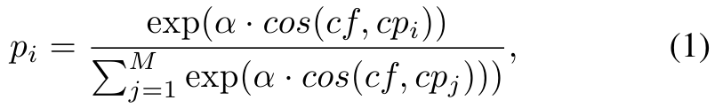
where α is the scaling factor. The cross entropy loss is utilized to optimize $p_i$ :
여기서 α는 스케일링 계수입니다. 교차 엔트로피 손실은 $p_i$ 를 최적화하는 데 사용됩니다.

D. Attribute representation learning

1) Prototype generation: We design a prototype generation module to perform the semantic-to-visual mapping from class and attribute semantics to their corresponding visual features.
1) 프로토 타입 생성 : 우리는 클래스 및 속성 의미론에서 해당 시각적 기능에 대한 의미론적 - 시각적 매핑을 수행하기 위해 프로토 타입 생성 모듈을 설계합니다.

It is a multilayer perceptron (MLP) with a few shared layers and two identical branches for class and attribute prototype generation, respectively.
MLP(다층 퍼셉트론)로, 각각 클래스 및 속성 프로토타입 생성을 위한 몇 개의 공유 레이어와 두 개의 동일한 브랜치가 있습니다.

The shared layers include two FC layers with the first followed by Relu.
공유 레이어에는 두 개의 FC 레이어가 포함되며 첫 번째 레이어와 Relu가 뒤따릅니다.

Each separate branch contains one FC, two Relus before and after the FC.
각 개별 분기에는 FC 전후에 두 개의 Relus와 하나의 FC가 있습니다.

Inspired by the class normalization (CN) in [15], which was introduced to preserve the variance of semantic-to-visual mapping, we follow its design to have two CN before the FC in each branch.
의미론적-시각적 매핑의 분산을 보존하기 위해 도입된 [15]의 클래스 정규화(CN)에서 영감을 받아, 우리는 각 분기의 FC 앞에 두 개의 CN을 가지도록 설계를 따른다.

CN can be seen as BatchNorm without the affine transform.
CN은 아핀 변환 없이 BatchNorm으로 볼 수 있다.

---

For attribute prototype generation, the input attribute semantics $AS$ are set as one-hot vectors such that $as_j$ only has its $j$-th value being nonzero in the vector.
속성 프로토타입 생성의 경우 입력 속성 의미 $AS$는 원핫 벡터로 설정되므로 $as_j$는 벡터 내에서 j번째 값만 0이 아닌 값을 갖는다.

AS can be seen as a basis to construct CS.
AS는 CS를 구성하는 기초라고 볼 수 있습니다.

Other orthogonal bases may also work to distinguish attributes whilst the one-hot form works the best empirically.
empirically 경험적으로
다른 직교 기반도 속성을 구별하는 데 사용할 수 있지만 one-hot 형식은 경험적으로 가장 잘 작동합니다.

AS are stored as a K × K matrix and fed into the prototype generation module to obtain AP.
AS는 K × K 행렬로 저장되고 프로토타입 생성 모듈에 공급되어 AP를 얻습니다.

Each ap is of C dimensions.
각 ap은 C 차원입니다.

Notice class prototype generation also utilizes this module which takes the input of CS and outputs CP.
주의 클래스 프로토타입 생성은 CS의 입력을 받아 CP를 출력하는 이 모듈도 활용합니다.

---

2) Attribute-level feature embedding.: For the extraction of attribute-level features, we follow [23], [26] to adopt an attention-based mechanism.
2) 속성 수준 특징 임베딩: 속성 수준 특징 추출을 위해 [23], [26]에 따라 주의 기반 메커니즘을 채택합니다.

By integrating it into our backbone architecture, we present the attention-based attribute localization scheme.
이를 백본 아키텍처에 통합하여 주의 기반 속성 지역화 체계를 제시합니다.

---

We first add four convolution layers after the last four residual blocks of the backbone (ResNet, R2∼R5) respectively to extract feature tensors of the same resolution H ×W ×K over multiple scales.
우리는 먼저 백본의 마지막 4개 잔여 블록(ResNet, R2~R5) 뒤에 각각 4개의 컨볼루션 레이어를 추가하여 여러 스케일에 걸쳐 동일한 해상도 H × W × K의 피쳐 텐서를 추출합니다.

These attention tensors $AM_s$ are pixel-wisely added together to produce the $AM$ , $AM = \sum ^4_{s=1}AM^s$ .
이러한 어텐션 텐서 $AM_s$는 픽셀 단위로 함께 추가되어 $AM$ , $AM = \sum ^4_{s=1}AM^s$ 를 생성합니다.

We apply the Softmax function on each feature map of $AM$ to move it in the range 0 to 1.
AM의 각 기능 맵에 Softmax 기능을 적용하여 0에서 1 범위로 이동합니다.

The feature map $am_j$ in AM hence serves as a soft mask indicating the potential localization of the j-th attribute.
indicate 나타내다 hence 따라서
따라서 AM의 형상 맵 $am_j$는 j-th 속성의 잠재적인 지역화를 나타내는 소프트 마스크 역할을 한다.

To obtain attribute-level features, we apply the bi-linear pooling between $AM$ and the image feature tensor $F$.
속성 수준 특징을 얻기 위해 AM과 이미지 특징 텐서 F 사이에 쌍선형 풀링을 적용합니다.

It is basically to apply each attribute-level soft mask to feature maps in F to localize this attribute [51].
기본적으로 각 속성 수준의 소프트 마스크를 F의 기능 맵에 적용하여 이 속성을 현지화하는 것입니다[51].

Specifically, each $am_j$ is pixel-wisely multiplied to every feature map $f_i$ in F followed by average pooling.
특히, 각 $am_j$는 평균 풀링이 뒤따르는 F의 모든 기능 맵 $f_i$에 픽셀 단위로 곱해집니다.

There are C feature maps in F , which ends up with a C-dimensional feature vector $af_j$ for the j-th attribute.
F에는 C 피쳐 맵이 있으며, 이는 j-th 속성에 대한 C 차원 피쳐 벡터 'afj'로 끝납니다.

The process can be written as,

where Softmax(·) is applied to the 2-dimensional (H × W ) input.
여기서 Softmax(·)는 2차원(H × W) 입력에 적용됩니다.

We use R(·) to expand $Softmax(am_j)$ (by replication) to C channels so as to pixel-wisely multiply with F ; $\odot$ is the element-wise product.
R(·)을 사용하여 $Softmax(am_j)$(복제에 의해)를 C 채널로 확장하여 F와 픽셀 단위로 곱합니다. $\odot$는 요소별 곱입니다.

By iterating $am_j$ over j, we obtain the final $AF = \{ af_j \}^K_{j=1}$.
iterate 반복하다
j에 대해 $am_j$를 반복하여 최종 $AF = \{ af_j \}^K_{j=1}$ 을 얻습니다.

---

3) Attribute representation optimization: Attribute-level features AF are extracted within each individual image, the features for the same attribute can vary in forms across many images.
3) 속성 표현 최적화: 속성 수준의 특징 AF는 각 개별 이미지 내에서 추출되며, 동일한 속성에 대한 특징은 여러 이미지에 걸쳐 형태가 다를 수 있습니다.

Attribute prototypes, on the other hand, are generated beyond images from orthogonal attribute semantics.
반면에 속성 프로토타입은 직교 속성 의미론의 이미지 너머에서 생성됩니다.

In order for the attribute representation optimization, we present two contrastive losses to let 1) any attribute-level feature be close to its corresponding attribute prototype; and 2) any attributelevel feature be close to other attribute-level features belonging to the same attribute.
속성 표현 최적화를 위해 1) 속성 수준 기능이 해당 속성 프로토타입에 가깝도록 두 가지 대조 손실을 제시합니다. 2) 모든 속성 수준 기능은 동일한 속성에 속하는 다른 속성 수준 기능에 가깝습니다.

---