1. Introduction

연구 배경

• scene에 대한 semantic, spatial, temporal structure를 추론하는 것은 자율주행에 있어서 중요한 task이다.

  ⇒ dynamic scene을 정확히 받아올 수 있다.

  • 이를 위해서, auxiliary(보조적인) task를 활용
    • 예를 들어, CILRS의 경우 simple self-supervised auxiliary training을 통해, ego-vehicle의 velocity를 예측했다.
  • NEAT는 auxiliary task로 BEV semantic prediction을 택했다.

• BEV semantic prediction

  

  • 과거, 미래에 대한 BEV semantic segmentation을 출력하는 model이 필요하다.
  • (x, y, t) ⇒ BEV spatiotemporal query location
    • ex) (2, 5, 2) ⇒ 2 meters in front of the vehicle, 5 meters to the right, 2 seconds into the future
    • 어떤 픽셀이 현재 location과 관련이 있는지 알기 어려움.
  • reasoning about 3D geometry, scene motion, ego-motion, interactions between scene elements 와 같은 정보들이 필요함

• NEAT ⇒ Neural Attention Fields for e2e driving

  • query location(x, y, t)과 interpretable attention map을 사용해서 해결

    

3. Method

Input & Output

Input

• Sensor data & Fixed length buffer of T time-steps
  • $\chi = \{ x_{s,t} \}_{s=1:S,t=1:T}$
    • S = 3 ⇒ forward, left, right RGB camera
      • full 180’ view
    • T = 1
• velocity : $v$
• Query point
  • (x, y, t, x’, y’) ⇒ 1 ≤ t ≤ T+Z
    • BEV spatiotemporal query location (x, y, t)마다 waypoint prediction, BEV semantic prediction을 수행한다.
    • (x’, y’)의 경우, target location으로써, waypoint prediction에 driver의 intention을 추가해서 조정해주는 역할을 한다.

Output

• Waypoint offset ⇒ $o_i$
  • (x_offset, y_offset) $\in \R^2$
• Semantic class ⇒ $s_i$

  • $s_i \in \R^K$ (K : class labels)

    

Architecture

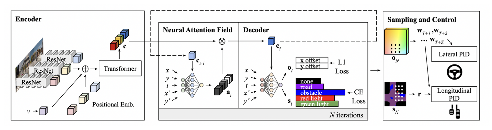
• $e_{\theta}$ : encoder
• $a_{\phi}$ : neural attention field
• $d_{\psi}$ : decoder

Encoder

• $e_{\theta} : \R^{S \times T \times W \times H \times 3} \times \R \rightarrow \R^{(S * T *P) \times C}$
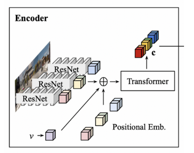
• Each Image : $x_{s, t} \in \R^{W \times H \times 3}$
• 각 센서, time-step 별 image들이 들어오면, ResNet backbone을 지나서 $\R^{P \times C}$와 같은 형태가 된다. 여기서, P는 image당 spatial feature의 갯수이고, C는 feature dimensionality이다. 결국, ResNet backbone을 지나면, $\R^{(S * T *P) \times C}$ 형태의 output으로 출력된다.
  
• 이 후에, velocity feature $v$, learned positional embedding을 더해서 Transformer에 Input으로 들어간다. ⇒ transformer의 self-attention mechanism을 통해 feature들을 global하게 통합해, 맥락적인 정보를 더 잘 받아오기 위함.
  • $v \rightarrow \R^C$ ⇒ obtained by linearly projectione
  • learned positional embedding : $\R^{(S*T*P) \times C}$
  • transformer의 output 또한 input과 동일하게 다음과 같이 출력된다.
  • $c \in \R^{(S*T*P) \times C}$

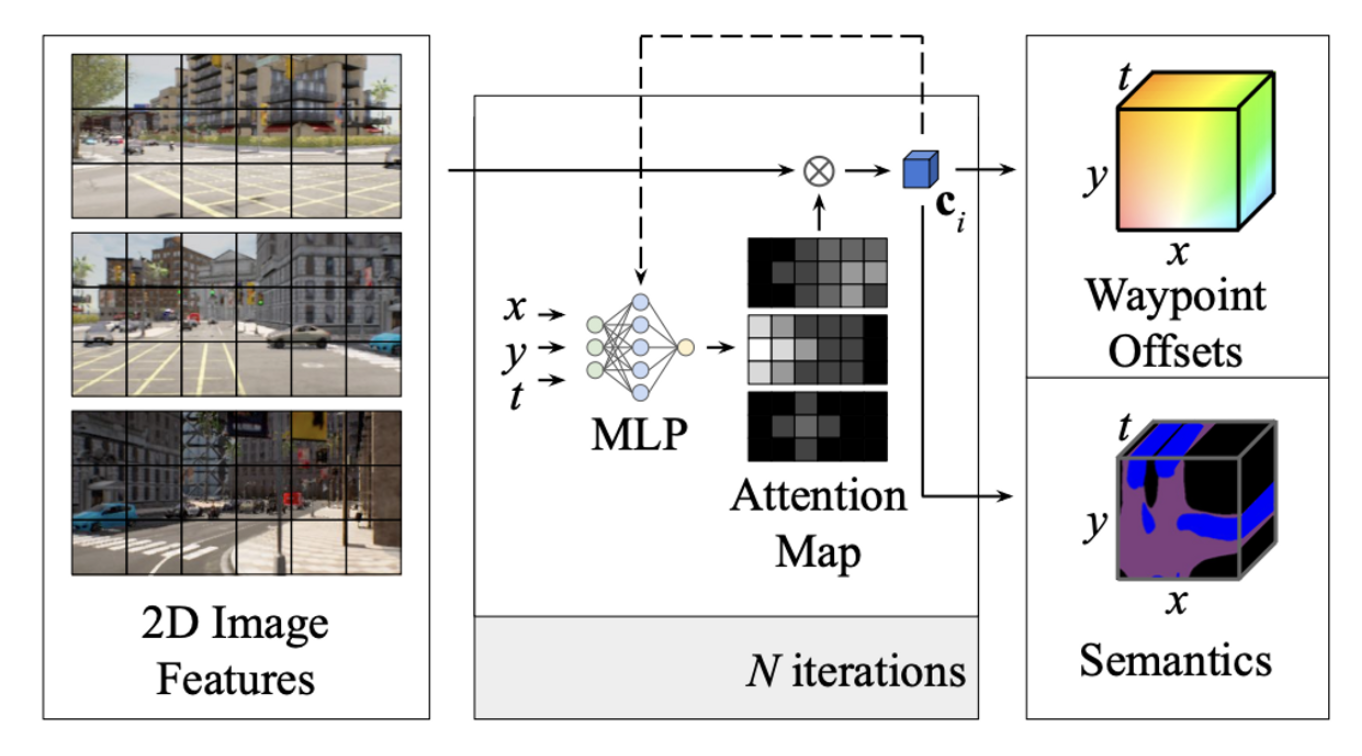
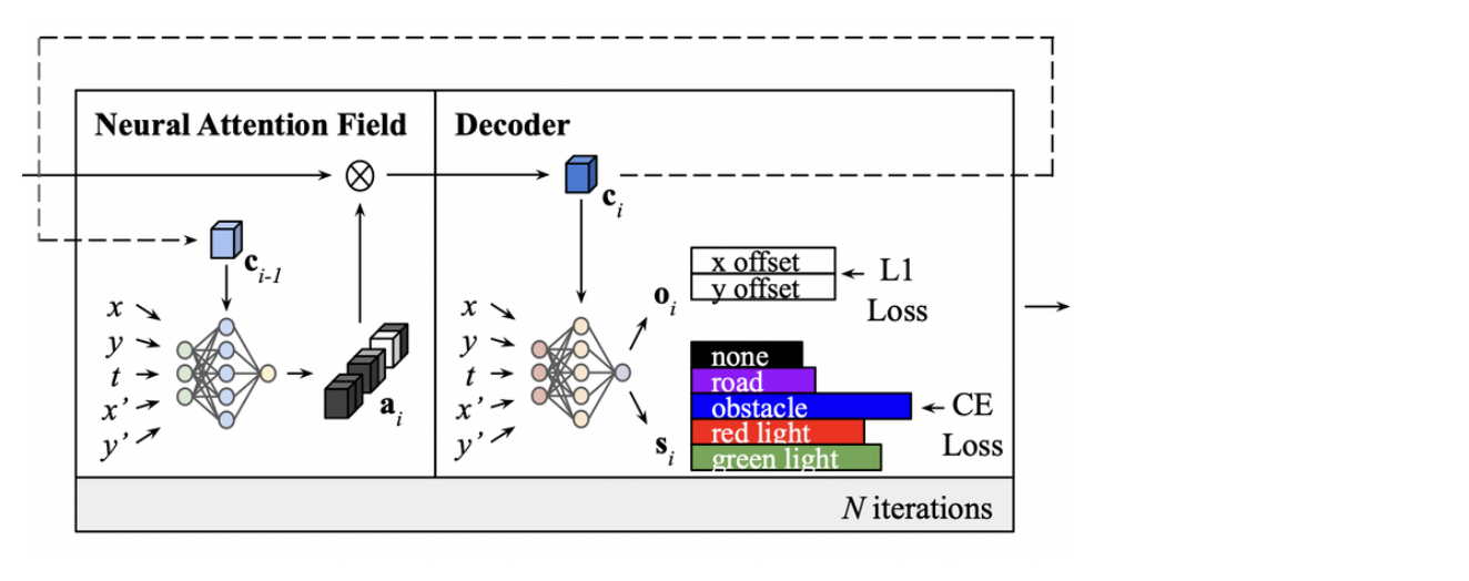
Neural Attention Field

• $a_{\phi} : \R^5 \times \R^C \rightarrow \R^{S *T*P}$

• query location은 $x, y, t$에 추가로 target location $(x', y')$가 추가되어, $\R^5$의 형태를 가진다.

• $c_i = softmax(a_i)^{\top} \cdot c$

  • $c_i \in \R^C$
  • $c_0$ : set to the mean of $c$

• MLP를 통해 attention map을 뽑아내는 과정은 다음과 같은 형태를 지닌다.

  

  • 5 fully-connected ResNet Block으로 구성되어 있으며, 중간에 $c_{i-1}$을 통해, CBN(conditional batch normalization)을 수행하는 구조로 이루어져 있다.

    • CBN?

      

      • $c_{i-1}$에 2-layer ReLU, MLP를 통해 128-dimensional vector $\beta_{b, 1}, \beta_{b,2},\gamma_{b,1}, \gamma_{b,2}$를 도출한다.

Decoder

• $d_{\psi} : \R^5 \times \R^C \rightarrow \R^K \times \R^2$
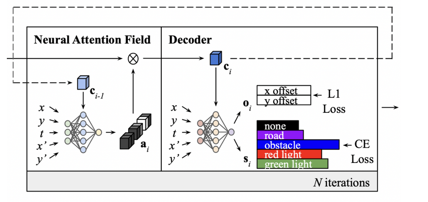
• $a_{\phi}$와 유사한 형태의 MLP 구조로 output layer에서 semantic class와 waypoint offset을 출력한다는 점이 다르다.
• 위 과정을 매 iteration마다 수행해 총 N번 수행한다.
  • But, intermediate iteration$(i < N)$은 test time에 이용되지 않음

Training

Sampling

• semantic class label의 경우, 보통 불균형하기 때문에, training 시기에 class-balancing sampling이 필요하다.
  • semantic class들 중에 가장 적은 point 갯수를 가지는 class 우선으로 $M \over K$point를 랜덤하게 추출된다.

Loss

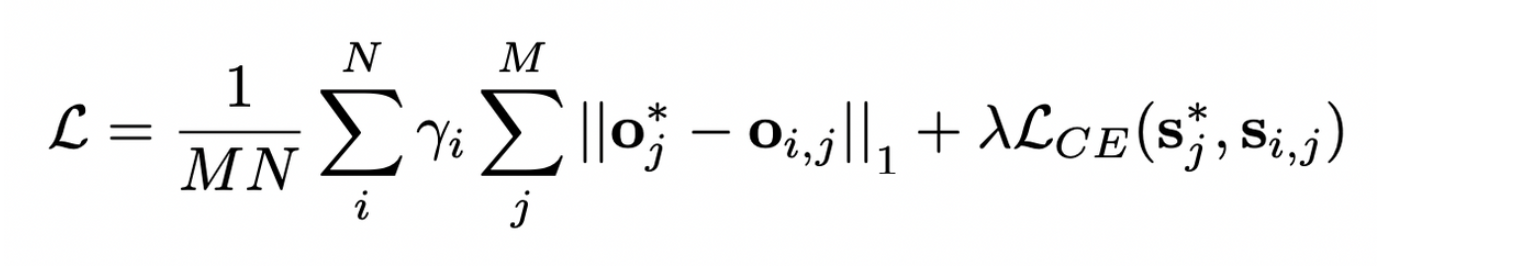
• waypoint offset loss의 경우, L1 Loss를, semantic class loss의 경우 Cross-Entropy Loss를 사용한다.
  • N : iterations
  • M : samples

Controller

• Red light indicator, waypoint를 구해서, 이를 PID controller를 이용해 steer, throttle, brake value로 변환한다.

Red Light Indicator ($r$)

• 현재 위치에서 정면 50m, 우측 25m 범위에 sparse grid sample point를 일정하게 찍어, 그 point의semantic prediction이 red light class인 것이 있다면, $r$을 1로 부여하고, 아니면 0으로 부여한다.
  • (U, V) grid ⇒ U = 16, V = 32

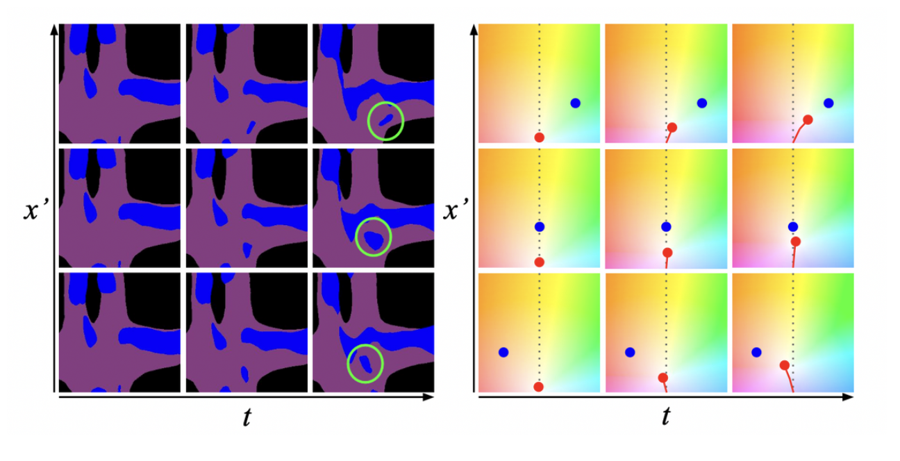
Waypoint

• 정면 A meter square 범위를 (G x G) grid point로 나누어, waypoint offset $o_N$을 각 $G^2$ grid point, 각 time-step(t=T+1, … , T+Z)에 더한다.
• 그 후에 모든 $G^2$ waypoint prediction의 average를 계산해 최종 waypoint prediction $w_t$를 구한다.

Experiments

Routes

• CARLA ver.0.9.10
• 42 routes from 6 different towns (training ⇒ 8 towns)
• 7 weathers
  • Clear, Cloudy, Wet, MidRain, WetCloudy, HardRain, SoftRain
• 6 daylight conditions
  • Night, Twilight, Dawn, Morning, Noon, Sunset

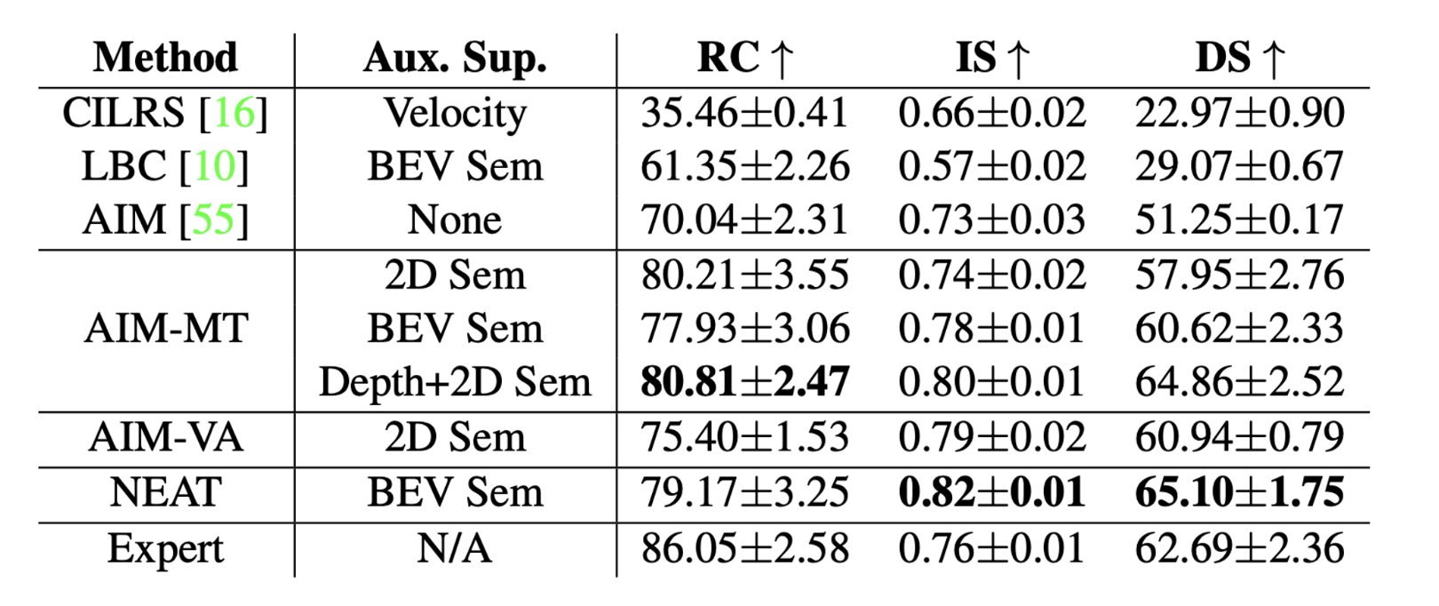
Metrics

• RC : Route Completion
• IS : Infraction Score
• DS : Driving Score

Driving Performance