기초 컴퓨터 비전: (8) Corresponding Points

고영민·2022년 2월 14일

SLAM: 기초 컴퓨터 비전부터 visual&LiDAR SLAM까지

목록 보기

14/17

앞선 내용에서 각 카메라의 orientation을 찾거나 촬영된 포인트의 3D 좌표를 복원하는 방법들을 알아보았다. 하지만 해당 과정에서 우리는 corresponding point(서로 다른 영상에서 중복되는 객체에 대한 점, 이전 글의 Figure 2. 참고)가 주어졌다고 가정하였는데, 이번 글에서는 이러한 corresponding point를 찾는 방법을 알아보고 기초 컴퓨터 비전 학습을 마무리한다.

1. Feature Extractor and Descriptor

Corresponding point를 찾기 위한 첫번째 방법으로 feature extractor(특징 추출자)와 descriptor(특징 기술자)의 조합을 들 수 있다. 먼저, feature extractor는 영상 내에서 어떠한 특징점을 찾아내는 것으로 영상 내에 나타나는 edge, corner 등이 대표적인 특징점이 될 수 있다. Feature descriptor는 이렇게 찾아낸 feature들마다 서로 구별되는 값을 할당하며, 이를 통해 두 영상에서 검출된 수많은 feature points 중 같은 point들을 짝지을 수 있다.

1.1. Extractor

1.1.1. Harris Corner Detector

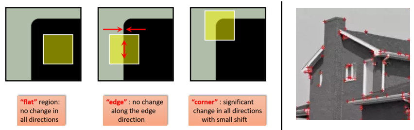
Harris corner detector는 입력 영상 내에서 모서리(corner)를 검출하는 방법이다. 기본적인 아이디어는 아래의 그림과 같이 모서리에서는 모든 방향에서의 픽셀값 변화가 크다는 점에 착안한다.

Figure 1. (좌) Harris corner detector 기본 원리, (우) Harris corner detector 예시

$I(x,y)$ 를 $(x,y)$ 에서의 image 픽셀값이라고 하면, $(x,y)$ 에서 미소 변화량 $(\delta x,\delta y)$ 만큼 변화시키면 영상의 변화량(여기서는 SSD(Sum of Squared Differences)사용)는 다음과 같이 쓸 수 있다.

f(x,y)=\sum_{(u,v) \in W_{xy}}{(I(x,y)-I(x+\delta x,y+\delta y))^2}

$I(x+\delta x,y+\delta y)$ 를 근사하기 위하여 Taylor 전개를 사용하면 픽셀값의 SSD 다음과 같이 쓸 수 있다.

\begin{aligned} f(x,y) & =\sum_{(u,v) \in W_{xy}}{(I(x,y)-\left(I(x,y)+ \begin{pmatrix} J_x & J_y \\ \end{pmatrix} \begin{pmatrix} \delta x\\ \delta y \end{pmatrix} \right))^2}\\ & \approx \sum_{(u,v) \in W_{xy}}{ \left(\begin{pmatrix} J_x & J_y \\ \end{pmatrix} \begin{pmatrix} \delta x\\ \delta y \end{pmatrix} \right)^2}\\ & = \sum_{(u,v) \in W_{xy}}{ \left( \begin{pmatrix} \delta x\\ \delta y \end{pmatrix}^T \begin{pmatrix} J_x^2 & J_xJ_y \\ J_xJ_y & J_y^2 \end{pmatrix} \begin{pmatrix} \delta x\\ \delta y \end{pmatrix} \right)}\\ & = \begin{pmatrix} \delta x\\ \delta y \end{pmatrix}^T \begin{pmatrix} \sum_W J_x^2 & \sum_W J_xJ_y \\ \sum_W J_xJ_y & \sum_W J_y^2 \end{pmatrix} \begin{pmatrix} \delta x\\ \delta y \end{pmatrix}\\ & =\begin{pmatrix} \delta x\\ \delta y \end{pmatrix}^T \mathbf{M} \begin{pmatrix} \delta x\\ \delta y \end{pmatrix} \end{aligned}

이때 사용된 $J$ 들은 Jacobian이며, 마지막 step에서 미소 변화량 $(\delta x,\delta y)$ 는 summation과 관계가 없기 때문에 밖으로 빼어 정리할 수 있다. 그리고 $\mathbf{M}$ 의 고윳값이 $\lambda_1 \ge \lambda_2$ 라면, 위와 같이 정리된 영상 변화량을 최대화하는 방향은 $\lambda_1$ 에 해당하는 고유벡터, 최소화하는 방향은 $\lambda_2$ 에 해당하는 고유벡터이다(변화량은 고유값).

$\mathbf{A}=\mathbf{A}^T=\mathbf{Q}\mathbf{\Lambda}\mathbf{Q}^T$ 이고, 행렬의 고유값이 $\lambda_1 \ge \cdots \ge \lambda_n$ 일 때, $\lambda_n \mathbf{x}^T\mathbf{x} \le \mathbf{x}^T\mathbf{A}\mathbf{x} \le \lambda_1 \mathbf{x}^T\mathbf{x}$ 가 성립

(증명)

\begin{aligned} \mathbf{x}^T\mathbf{A}\mathbf{x} & =\mathbf{x}^T\mathbf{Q}\mathbf{\Lambda}\mathbf{Q}^T\mathbf{x}\\ & = (\mathbf{Q}^T\mathbf{x})^T\mathbf{\Lambda}(\mathbf{Q}^T\mathbf{x})\\ & = \sum_{i=1}^{n}{(\lambda_i q^T_i \mathbf{x})^2}\\ & \ge \lambda_1 \sum_{i=1}^{n}{(q^T_i \mathbf{x})^2}\\ & = \lambda_1 |\mathbf{x}|^2 \end{aligned}

2번째 step에서 3번째 step으로 넘어가는 과정은 $\Lambda$ 가 대각행렬이라는 점과 $\mathbf{Q}^T$ 의 행벡터를 쪼개어 생각하면 알 수 있으며, 4번째 step에서 5번째 step은 $\mathbf{Q}$ 가 직교행렬이라는 점에서 알 수 있다.

위의 결과를 통해 $\mathbf{x}^T\mathbf{A}\mathbf{x} \le \lambda_1 \mathbf{x}^T\mathbf{x}$ 를 알 수 있고, 반대쪽도 비슷한 과정으로 유도할 수 있다.

$\mathbf{x}$ 가 $\lambda_1$ 에 해당하는 고유벡터일 때, $\mathbf{x}^T\mathbf{A}\mathbf{x} = \lambda_1 \mathbf{x}^T\mathbf{x}$ 와 같이 등호가 성립한다.

따라서 두 고유값이 모두 클 때가 corner라는 것을 유추할 수 있으며, 어떤 행렬에서 행렬값은 고유값들의 곱, trace는 고유값들의 합인 점을 사용하여 다음과 같은 criterion 식을 만들 수 있다.

\begin{aligned} R & = det(\mathbf{M}) - k(tr(\mathbf{M}))^2\\ & = \lambda_1\lambda_2 -k(\lambda_1 + \lambda_2)^2 \end{aligned}

여기서 $k$ 는 0.04~0.06 정도의 작은 상수를 사용하며, 위의 값에 따라 다음과 같이 분류할 수 있다.

\begin{cases} |R| \approx 0 \rightarrow \lambda_1 \approx \lambda_2 \approx 0 : flat \; region\\ |R| \lt 0 \rightarrow \lambda_1 \gg \lambda_2 \; or \; \lambda_2 \gg \lambda_1 : edge\\ |R| \gg 0 \rightarrow \lambda_1 \approx \lambda_2 \gg 0 : corner \end{cases}

여기서 Harris corner detector는 사용하기에 따라 edge도 검출이 가능하다는 점을 알 수 있다.

마지막으로 $\mathbf{M}$ 을 얻기 위하여 Jacobian을 구할 필요가 있는데 이는 Scharr 또는 Sobel 필터와의 convolution 연산을 통해 구할 수 있다.

1.1.2. FAST(Features from Accelerated Segment Test)

1.2. Descriptor

1.2.1. SIFT(Scale-Invariant Feature Transform)

1.2.1. BRIEF(Binary Robust Independent Elementary Features)

2. Stereo Matching

Feature extractor와 descriptor의 조합은 각 입력 영상에 대해서 독립적으로 작동하여 특징점을 추출하고 그에 해당하는 기술자를 서로 비교하여 corresponding points를 찾는다면, stereo matching에서는 두 장의 image가 동시에 주어지며 하나의 image에서 얻은 작은 크기의 patch를 다른쪽 image에서 일일이 비교하며 가장 유사한 위치를 찾는 방법이다.

2.1 Matching

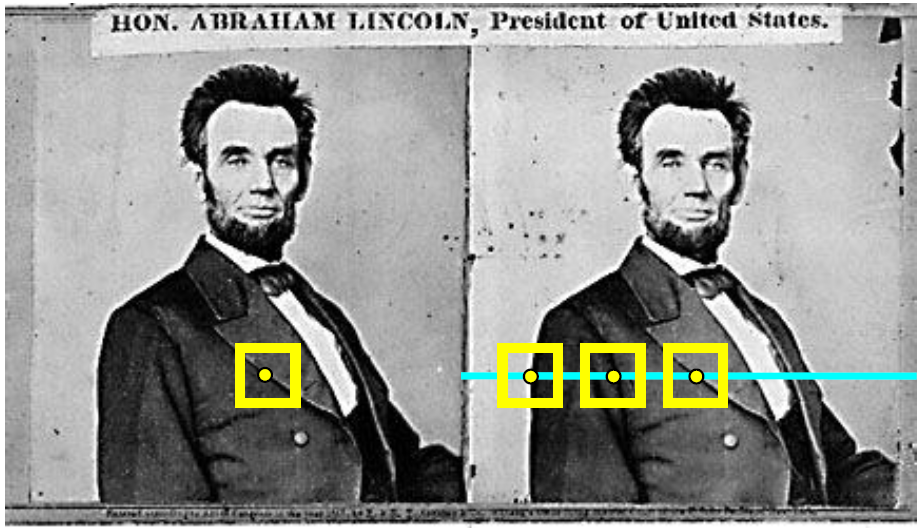
Figure 2. Stereo matching

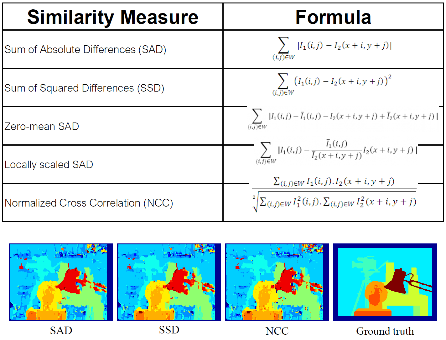
Figure 2.는 stereo matching 방법을 보여주며, 왼쪽에서 뽑아낸 patch(노란색 박스)와 가장 유사한 부분을 오른쪽 그림에서 찾기 위해 여러 위치에 대해서 patch를 뽑아내서 서로 비교한다. 이를 위하여 두 patch를 비교하여 유사도를 계산할 수 있는 식이 필요한데 다음과 같이 여러 종류의 식을 사용할 수 있다.

Figure 3. Stereo matching에서 사용 가능한 여러 measure

다만, 유사한 patch를 찾기 위하여 image 내의 모든 위치에 대해서 탐색을 하면 연산 시간이 너무 오래걸린다. 이러한 연산 시간을 줄이기 위하여 보통 epipolar line 상의 위치에 대해서만 탐색을 하는데, 이전 글에서 알 수 있듯이, corresponding points들은 하나의 epipolar plane 상에 위치하기 때문에 이러한 탐색 방법이 성립하게된다.

2.2 Rectification

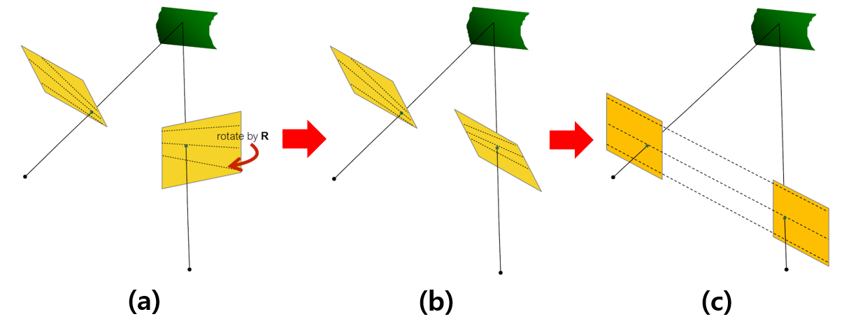
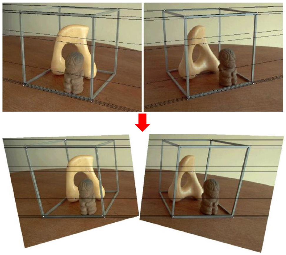
두 영상이 입력되었을 때, 일반적으로는 아래 그림의 (a)와 같이 epipolar line이 정렬되지 않은 상태이다. 만약 matching을 수행하고자 하는 부분이 많다면 그 때마다 epipolar line을 구하는 것은 연산량을 많이 낭비하게 된다. Rectification은 이러한 문제를 해결하기 위한 전처리 과정으로 아래 그림과 같이 epipolar line이 평행하게 정렬되도록 두 이미지를 변환한다.

Figure 4. Rectification 과정

Rectification을 수행하기 위하여, 먼저 essential matrix에서 두 영상 사이의 rotation matrix $\mathbf{R}$ 을 구하며, 이 과정은 이전 글에 나와있다. 해당 rotation matrix을 두번째 영상에 가하면 두 영상은 Fig 4.의 (b)처럼 같은 방향을 바라보게 된다.

그 다음으로 epipolar line들을 평행하게 변환하기 위하여 epipole을 무한대 점으로 보낸다. 이를 위한 회전행렬 $\mathbf{R_{rect}}$ 는 다음과 같다.

\mathbf{R_{rect}}= \begin{pmatrix} \mathbf{r_1}^T\\ \mathbf{r_2}^T\\ \mathbf{r_3}^T \end{pmatrix}, \;\;\;\;\; \begin{cases} \mathbf{r_1} = \mathbf{e_1} = \mathbf{b}/|\mathbf{b}|\\ \mathbf{r_2} = \frac{[-b_y \;\;\; b_x \;\;\;0]}{\sqrt{b_x^2 + b_y^2}} \\ \mathbf{r_3} = \mathbf{r_1} \times \mathbf{r_2} \end{cases}

이때, $\mathbf{R_{rect}}\mathbf{e_1}=(1,0,0)^T$ 이 되어 무한대로 가는 것을 확인할 수 있으며, epipole $\mathbf{e_1}$ 는 반대편 카메라 중심이 투영된 점이므로 essential matrix에서 복원한 translate $\mathbf{b}$ 를 통해 구할 수 있다. 따라서 전체적인 알고리즘은 다음과 같다.

Figure 5. Image rectification 알고리즘

Figure 6. Image rectification 결과

3. Optical Flow & Tracking

이 방법은 영상에서 픽셀의 변화를 기반으로 움직임을 예측 및 추적하는 방법으로, 이를 위하여 image의 gradient를 계산하게 된다.

3.1. Optical Flow

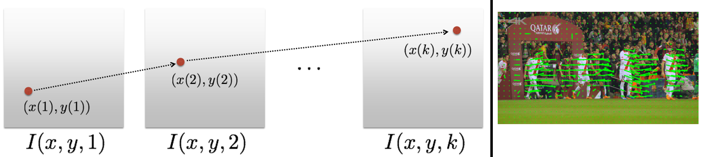
Optical flow는 시간 경과에 따른 pixel들의 움직임을 계산하는 방법으로 대표적인 방법으로 Lucas-Kanade 방법이 있다. 이러한 optical flow를 사용하면 특징점의 움직임이나 image pixel 전체의 움직임을 추적할 수 있다. 아래의 그림을 보면 optical flow를 적용함으로써 움직이는 객체(축구선수)에 대한 픽셀을 추적할 수 있다.

Figure 7. Optical flow의 개념과 적용 결과

Optical flow 방법은 몇 가지 가정을 하여 식을 유도하며, 첫번째로 같은 객체에 대한 포인트의 픽셀값은 시간이 지나더라도 같으며(즉 위 그림에서 빨간 점에 대한 픽셀값은 모두 같음), 두번째로 픽셀의 움직임이 작아 시간에 따른 위치 변화를 $(x+u\delta t, y+v\delta t)$ 와 같이 선형적으로 쓸 수 있다는 것이다( $(u,v)$ 는 optical flow에서 사용하는 픽셀의 속도). 이를 종합하면 다음과 같이 쓸 수 있다.

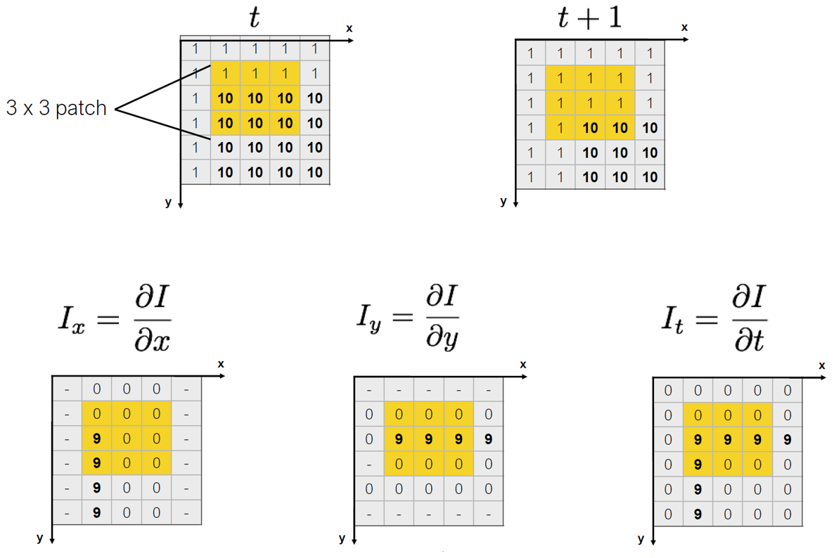
I(x+u\delta t, y+v\delta t, t+\delta t)=I(x,y,t)

위의 식을 선형화하기 위하여 1차 Taylor 전개를 적용하면 다음과 같다.

I(x+u\delta t, y+v\delta t, t+\delta t)=I(x,y,t) + \frac{\partial I}{\partial x}dx + \frac{\partial I}{\partial y}dy + \frac{\partial I}{\partial t}dt

이 식을 대입하면 다음과 같다.

\frac{\partial I}{\partial x}dx + \frac{\partial I}{\partial y}dy + \frac{\partial I}{\partial t}dt = 0

\frac{\partial I}{\partial x}\frac{dx}{dt} + \frac{\partial I}{\partial y}\frac{dy}{dt} = -\frac{\partial I}{\partial t}

\begin{pmatrix} I_x & I_y \end{pmatrix} \begin{pmatrix} u \\ v \end{pmatrix} = -I_t

여기서 $I_x, I_y$ 는 각각 image $I$ 에서 $x, y$ 방향의 gradient이다. 이러한 image gradient는 다음 그림과 같으며, Harris corner detector에서도 언급하였듯이 Scharr 또는 Sobel 필터와의 convolution 연산을 통해 구할 수 있다.

Figure 8. Image gradient

Optical flow의 목표는 픽셀의 속도인 $(u,v)$ 를 찾는 것으로, 미지수가 2개이므로 이를 결정하기 위하여 contraint가 더 필요하다. Lucas-Kanade 방법에서는 추가적으로 한 patch내에서는 모든 픽셀이 같은 속도를 갖는다는 가정을 추가하여 식을 세운다.

해당 가정 상에서 만약 $5 \times 5$ patch를 사용한다면 다음과 같이 25개의 식을 세울 수 있다.

\begin{pmatrix} I_{x, 1} & I_{y, 1} \\ \vdots\\ I_{x, n} & I_{y, n} \end{pmatrix} \begin{pmatrix} u \\ v \end{pmatrix} = \begin{pmatrix} I_{t, 1} \\ \vdots\\ I_{t, n} \end{pmatrix} \rightarrow \mathbf{A}\mathbf{x}=\mathbf{b}

해당 식은 SVD 등을 통한 least squre 문제로 해결해도 되며, 가능하다면 $\mathbf{A}\mathbf{x}=\mathbf{b} \rightarrow \mathbf{A}^T\mathbf{A}\mathbf{x}=\mathbf{A}^T\mathbf{b} \rightarrow \mathbf{x}=(\mathbf{A}^T\mathbf{A})^{-1}\mathbf{A}^T\mathbf{b}$ 과 같이 풀 수도 있다. 만약 $\mathbf{A}$ 의 column vector들이 일차독립이라면 QR decomposition이 가능하여 $\mathbf{A}^T\mathbf{A}=(\mathbf{Q}\mathbf{R})^T\mathbf{Q}\mathbf{R}=\mathbf{R}^T\mathbf{Q}^T\mathbf{Q}\mathbf{R}=\mathbf{R}^T\mathbf{R}$ 인데, $\mathbf{R}$ 은 삼각행렬로 가역행렬이므로 $\mathbf{R}^T\mathbf{R}=\mathbf{A}^T\mathbf{A}$ 또한 가역행렬이다. 위의 optical flow 문제에서 $\mathbf{A}$ 의 행은 2개 밖에 안되어 대부분의 경우 두 행이 선형 독립일 것이며, $\mathbf{A}^T\mathbf{A}$ 는 $2 \times 2$ 행렬이므로 $(\mathbf{A}^T\mathbf{A})^{-1}\mathbf{A}^T\mathbf{b}$ 를 구하는 것이 더 편리할 것이다.

3.2. Tracking

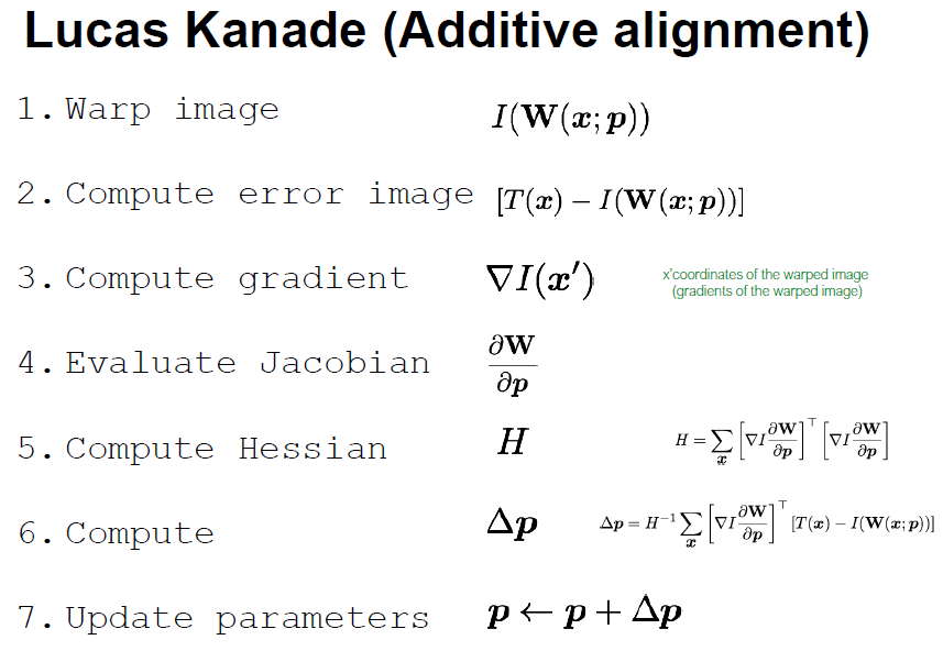
Optical flow가 image gradient를 기반으로 특정 위치의 픽셀 움직임을 예측하는 방법이었다면, tracking은 다음과 같은 식 처럼 어떤 template image를 warping하여 가장 일치하는 부분을 찾는 방법이다.

\min_\mathbf{p}\sum_\mathbf{x}{(I(W(\mathbf{x};\mathbf{p}))-T(\mathbf{x}))^2}

여기서 $\mathbf{x}$ 는 영상 내 픽셀 좌표, $\mathbf{p}$ 은 transform parameter, $W$ 는 image warping 함수(trasformation이라고 보면 됨), $I, T$ 는 각각 원래 이미지와 template 이미지이다. 위의 식은 같은 객체가 촬영되었다면 다른 시점에서 촬영되어도 같은 픽셀값을 같는다는 불변성 가정에 기반한다.

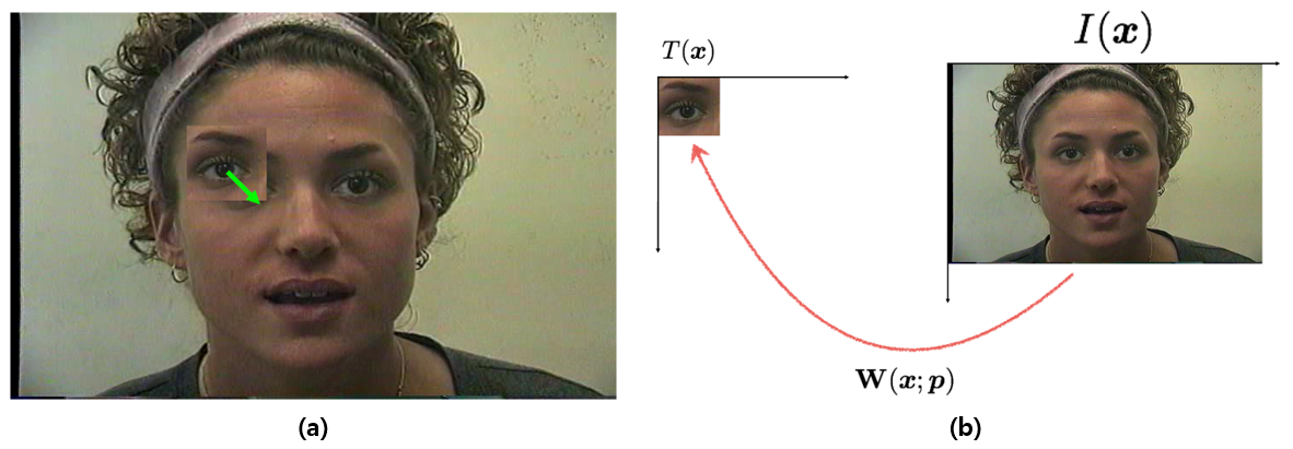
Track 문제는 아래 그림과 같이 볼 수 있으며, 하나의 template image가 주어지고 연속적인 입력영상이 주어질 때마다 적절한 $\mathbf{p}$ 를 찾을 수 있다면, template image에 해당하는 객체의 위치를 지속적으로 추적할 수 있다.

Figure 9. (a) tracking의 목적, template image의 위치를 찾아내어 추적함, (b) tracking 문제

우리가 원하는 것은 위의 식을 만족하는 $\mathbf{p}$ 를 찾는 것이지만, $\mathbf{p}$ 가 들어있는 함수 $I$ 가 non-parametric 함수(paramter로 표현할 수 없는 함수, $I$ 는 입력 위치에 대한 영상의 intensity 값을 반환하는 함수이므로 특별한 식으로 표현할 수 없음)이고 전체식에 제곱을 취하여 linear하지도 않다. 따라서 위의 식을 풀기 위하여 주어진 식을 선형화하는 작업이 필요하며, 이를 위해 먼저 $\mathbf{p}$ 에 대한 적당한 initial guess가 주어졌다고 가정하여 아래와 같이 쓴다.

\min_\mathbf{p}\sum_\mathbf{x}{(I(W(\mathbf{x};\mathbf{p}))-T(\mathbf{x}))^2} \;\;\; \rightarrow \;\;\; \min_\mathbf{p}\sum_\mathbf{x}{(I(W(\mathbf{x};\mathbf{p}+\Delta \mathbf{p}))-T(\mathbf{x}))^2}

여기서 우리는 $I(W(\mathbf{x};\mathbf{p}+\Delta \mathbf{p}))$ 에 Taylor 전개를 적용할 수 있으며, 1차 Taylor 전개를 적용하면 다음과 같다.

\begin{aligned} I(W(\mathbf{x};\mathbf{p}+\Delta \mathbf{p})) & \approx I(W(\mathbf{x};\mathbf{p})) + \frac{\partial I(W(\mathbf{x};\mathbf{p}))}{\partial \mathbf{p}}\Delta \mathbf{p} \\ & = I(W(\mathbf{x};\mathbf{p})) + \frac{\partial I(W(\mathbf{x};\mathbf{p}))}{\partial \mathbf{x'}} \frac{\partial W(\mathbf{x};\mathbf{p})}{\partial \mathbf{p}} \Delta \mathbf{p} \\ & = I(W(\mathbf{x};\mathbf{p})) + \nabla I \frac{\partial W}{\partial \mathbf{p}} \Delta \mathbf{p} \end{aligned}

여기서 $\mathbf{x'}=W(\mathbf{x};\mathbf{p})$ 이다. 위의 Taylor 전개를 목표식에 적용하면 다음과 같다.

\begin{aligned} \min_\mathbf{p}\sum_\mathbf{x}{(I(W(\mathbf{x};\mathbf{p}+\Delta \mathbf{p}))-T(\mathbf{x}))^2} & \approx \min_\mathbf{p}\sum_\mathbf{x}{\left( I(W(\mathbf{x};\mathbf{p})) + \nabla I \frac{\partial W}{\partial \mathbf{p}} \Delta \mathbf{p}-T(\mathbf{x})\right)^2}\\ & = \min_\mathbf{p}\sum_\mathbf{x}{ \left( \nabla I \frac{\partial W}{\partial \mathbf{p}} \Delta \mathbf{p} - [T(\mathbf{x}) - I(W(\mathbf{x};\mathbf{p}))] \right)^2}\\ & = \min_\mathbf{p} |\mathbf{A}\mathbf{p}-\mathbf{b}|^2 \end{aligned}

결과적으로 $\mathbf{A}=\nabla I \frac{\partial W}{\partial \mathbf{p}}$ , $\mathbf{b}=[T(\mathbf{x}) - I(W(\mathbf{x};\mathbf{p}))]$ 로 두었을 때 목표식이 least square 문제가 되며, 앞에서 이 문제의 해는 $(\mathbf{A}^T\mathbf{A})^{-1}\mathbf{A}^T\mathbf{b}$ 로 주어짐을 보았다. 따라서 해는 다음과 같이 쓸 수 있다.

\Delta\mathbf{p} = H^{-1}\sum_\mathbf{x}{\left[ \nabla I \frac{\partial W}{\partial \mathbf{p}} \right]^T}[T(\mathbf{x}) - I(W(\mathbf{x};\mathbf{p}))] \;\;\;\;\;\;\;\; \cdots (\mathbf{A}^T\mathbf{A})^{-1}\mathbf{A}^T\mathbf{b}

H = \sum_\mathbf{x}{\left[ \nabla I \frac{\partial W}{\partial \mathbf{p}} \right]^T}\left[ \nabla I \frac{\partial W}{\partial \mathbf{p}} \right] \;\;\;\;\;\;\;\; \cdots \mathbf{A}^T\mathbf{A}

이렇게 최적의 $\Delta\mathbf{p}$ 를 구할 수 있었지만, 사실 처음의 initial guess가 부정확하다면 한번에 정확한 위치를 알아내기 어려울 수 있다. 이러한 문제를 해결하기 위해 $\mathbf{p}_{i+1} \leftarrow \mathbf{p}_i +\Delta\mathbf{p}$ 와 같이 업데이트하고 같은 과정을 반복하여 더욱 정확한 위치를 찾을 수 있다.

이러한 방법을 Lucas-Kanade alignment라고 하며, 전체적인 알고리즘은 다음과 같다.

Figure 10. Lucas-Kanade alignment 알고리즘

이제 이러한 alignment 알고리즘을 변화하는 영상에 대해서 지속적으로 수행하면 tracking이 가능하다.

4. Motion Field

Optical flow가 이미지의 픽셀값이 어떻게 변화하는 지(image gradient 등)를 통해 픽셀의 움직임을 추정한다면, Motion Field는 실제로 촬영되는 객체와 카메라의 상대적인 motion(3D)를 알고있을 때, 해당 motion을 2D image plane에 투영하여 픽셀의 움직임을 추정하는 방법이다.

만약 정지해 있는 객체를 촬영할 때 조명이 변화한다고 가정했을 때, optical flow의 경우 어떤 값을 출력하지만, motion field는 0이 된다.

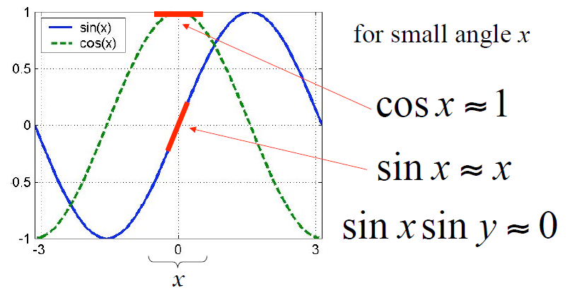
이전 글과 같이 3D에서의 회전행렬을 정의할 수 있고, 이를 모두 곱해보면 다음과 같다.

R^{3D}(\Psi, \phi, \theta) = R_z(\Psi)R_y(\phi)R_x(\theta) = \begin{pmatrix} \cos\Psi \cos\phi & -\sin\Psi\cos\theta + \cos\Psi\sin\phi\sin\theta & \sin\Psi\sin\theta + \cos\Psi \cos\theta \sin\phi \\ \sin\Psi \cos\phi & \cos\Psi \cos\theta + \sin\theta\sin\phi\sin\Psi & -\cos\Psi\sin\theta + \sin\phi\sin\Psi\cos\theta \\ -\sin\phi & \cos\phi \sin\theta & \cos\phi \cos\theta \end{pmatrix}

다만 카메라 영상에서 연속된 두 프레임 사이의 시간 차이는 매우 짧은 경우가 대부분이므로 회전 각도가 작은 편이며, 다음과 같이 근사할 수 있다.

Figure 11. Small angle approximation

해당 근사를 이용하면, 회전 행렬을 다음과 같이 간단하게 표현할 수 있다.

R^{3D}(\Psi, \phi, \theta) \approx \begin{pmatrix} 1 & -\Psi & \phi \\ \Psi & 1 & -\Psi \\ -\phi & \theta & 1 \end{pmatrix} = \mathbf{I}+ \begin{pmatrix} 0 & -\Psi & \phi \\ \Psi & 0 & -\theta \\ -\phi & \theta & 0 \end{pmatrix} = \mathbf{I}+\hat{\mathbf{s}}

여기서 $\mathbf{s}=(\theta, \phi, \Psi)^T$ 이다.

3D에서 어떤 물체 $\mathbf{P}$ 가 이동할 때, 그 변위는 $\mathbf{d}=\mathbf{R}\mathbf{P}+\mathbf{T}-\mathbf{P}$ 이며, 작은 각도를 가정한다면, $\mathbf{d}=(\mathbf{I}+\hat{\mathbf{s}})\mathbf{P}+\mathbf{T}-\mathbf{P}=\hat{\mathbf{s}}\mathbf{P}+\mathbf{T}$ 가 된다. 이때, 시간 간격이 충분히 작다면 위의 식을 변위가 아닌 속도에 대한 식으로도 사용 가능하며, 다음과 같다.

\mathbf{V} = \mathbf{T} + \mathbf{\omega} \times \mathbf{P}

여기서 $\mathbf{V}$ 는 물체의 속도, $\mathbf{T}$ 는 물체의 선속도 $\mathbf{\omega}=(\omega_x, \omega_y, \omega_z)^T$ 는 물체의 각속도이다. 만약, 물체가 정지해 있고 카메라가 위와 같이 움직인다면, 카메라의 시점에서 물체가 $\mathbf{V} = -\mathbf{T} - \mathbf{\omega} \times \mathbf{P}$ 와 같이 움직이는 것으로 보인다. 이는 부호만 변경된 식이며, 여기서는 이 식을 사용한다.

$\mathbf{V} = -\mathbf{T} - \mathbf{\omega} \times \mathbf{P}$ 을 성분 별로 풀어쓰면 다음과 같다.

\begin{cases} V_x = -\mathbf{T}_x - \mathbf{\omega}_y Z + \mathbf{\omega}_z Y \\ V_y = -\mathbf{T}_y - \mathbf{\omega}_z X + \mathbf{\omega}_x Z \\ V_z = -\mathbf{T}_z - \mathbf{\omega}_x Y + \mathbf{\omega}_y X \end{cases}

$\mathbf{P}$ 가 카메라 투영에 의해 픽셀 $\mathbf{p}$ 에 매핑된다고 할 때, $\mathbf{p}=f\mathbf{P}/Z$ 이다. 이를 미분하여 속도의 매핑식을 구하면 다음과 같다.

\begin{aligned} \frac{d\mathbf{p}}{dt}=\mathbf{v}=\frac{d\frac{f\mathbf{P}}{Z}}{dt} & =\frac{f}{Z^2}\left[ \frac{d\mathbf{P}}{dt}Z -\mathbf{P}\frac{dZ}{dt} \right] \\ & = \frac{f}{Z^2}\left[ \mathbf{V}Z-\mathbf{P}V_z \right] \\ & = f\frac{\mathbf{V}}{Z} - \mathbf{p}\frac{V_z}{Z} \end{aligned}

이를 성분 별로 풀어쓰면 다음과 같다.

\begin{cases} v_x = f\frac{V_x}{Z} - x\frac{V_z}{Z} \\ v_y = f\frac{V_y}{Z} - y\frac{V_z}{Z} \\ v_z = 0 \end{cases}

여기서 픽셀은 image plane 위에 있기 때문에 $z$ 방향 속력은 0이며, 이제 두 식을 합쳐서 $v_x, v_y$ 를 각속도, 선속도, 픽셀 위치에 대한 식으로 쓰면 다음과 같다.

\begin{cases} v_x = \frac{T_z x-T_x f}{Z} - \omega_y f + \omega_z y+\frac{\omega_x xy}{f}-\frac{\omega_y x^2}{f} \\ v_y = \frac{T_z y-T_y f}{Z} + \omega_x f - \omega_z x - \frac{\omega_y xy}{f} + \frac{\omega_x y^2}{f} \end{cases}

이것이 motion field 식이며, 때때로 $f=1$ 로 normalize하고 위의 식을 다음과 같이 행렬로 나타내기도 한다.

\begin{pmatrix} \Delta x \\ \Delta y \end{pmatrix} = \frac{1}{Z} \begin{pmatrix} -1 & 0 & x \\ 0 & -1 & y \end{pmatrix} \begin{pmatrix} T_x \\ T_y \\ T_z \end{pmatrix} + \begin{pmatrix} xy & -(1+x)^2 & y \\ (1+y)^2 & -xy & -x \end{pmatrix} \begin{pmatrix} R_x \\ R_y \\ R_z \end{pmatrix}

5. RANSAC(RANdom SAmple Consensus)

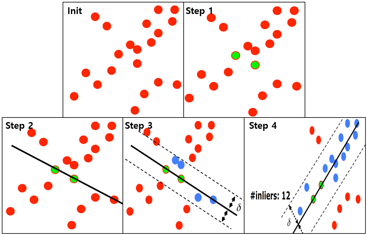
보통 corresponding points를 찾을 때 feature extractor & descriptor나 feature extractor & optical flow(or tracker) 등의 조합을 사용할 경우 굉장히 많은 수의 point를 검출하게 된다. 또한 굳이 computer vision 분야 뿐만 아니라 수많은 데이터가 주어졌을 때 해당 데이터에 노이즈가 섞여있다면 해당 데이터를 완벽히 설명하는 모델을 만드는 것이 불가능하기 때문에 최대한 많은 수의 데이터를 잘 설명할 수 있는 모델을 찾게된다. RANSAC 알고리즘은 이러한 목적을 위해 사용되며, 다음과 같은 과정으로 이루어져 있다.