Sampling from EBMs: Unadjusted Langevin MCMC

Unadjusted Lagevin MCMC는 다음과 같은 process를 거친다.

1. $\mathbf{x}^0\sim\pi(\mathbf{x})$
2. Repeat for $t=0,1,2,\cdots,T-1$
   • $\mathbf{z}^t\sim\mathcal{N}(0,I)$
   • $\mathbf{x}^{t+1}=\mathbf{x}^t+\epsilon\nabla_\mathbf{x}\log p_\theta(\mathbf{x})|_{\mathbf{x=x}^t}+\sqrt{2\epsilon}\mathbf{z}^t$

$\mathbf{x}^T$는 $p_\theta(\mathbf{x})$의 sample로 convergence 하는 것이 보장되어있으며, $\nabla_\mathbf{x}\log p_\theta(\mathbf{x})=\nabla_\mathbf{x}f_\theta(\mathbf{x})$ 이다. ($Z(\theta)$는 0이 되기 때문) 그러나 $\mathbf{x}$의 dimension이 커질 수록 convergence는 점점 느려진다. 문제는 energy based models를 학습할 때 contrastive divergence를 이용하면 sampling이 필요하다는 것이다. 따라서 느린 sampling 속도는 매우 치명적이다.

Score Matching

Energy-based model $p_\theta(\mathbf{x})=\frac{\exp\{f_\theta(\mathbf{x})\}}{Z(\theta)},\log p_\theta(\mathbf{x})=f_\theta(\mathbf{x})-\log Z(\theta)$가 주어졌을 때, score function은 다음과 같이 정의 된다.

• score function $s_\theta(\mathbf{x}):=\nabla_\mathbf{x}\log p_\theta(\mathbf{x})=\nabla_\mathbf{x}f_\theta(\mathbf{x})-\nabla_\mathbf{x}\log Z(\theta)=\nabla_\mathbf{x}f_\theta(\mathbf{x})$

위 식에서 알수 있듯이, score function은 partition function을 신경 쓰지 않아도 된다.

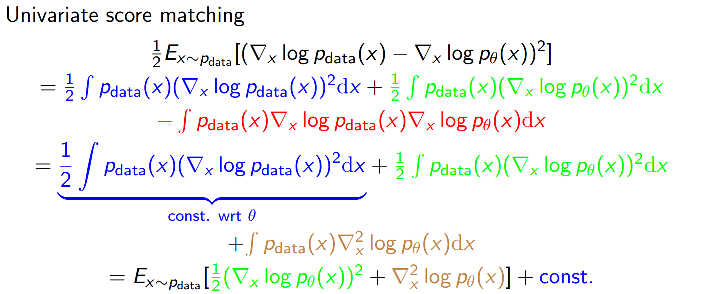
Fisher divergence를 이용하면 score function을 이용한 학습이 가능하다. 이를 score matching이라고 한다.

• Fisher divergence
  $D_F(p,q):=\frac{1}{2}E_{\mathbf{x}\sim p}[||\nabla_\mathbf{x}\log p(\mathbf{x})-\nabla_\mathbf{x}\log q(\mathbf{x})||_2^2]$
• score matching
  $\frac{1}{2}E_{\mathbf{x}\sim p_{data}}[||\nabla_\mathbf{x}\log p_{data}(\mathbf{x})-s_\theta(\mathbf{x})||^2_2]$

위 식은 $\log p_{data}(\mathbf{x})$ 을 알수 없기 때문에 문제가 된다. 따라서 $\log p_{data}(\mathbf{x})$를 계산하지 않는 트릭이 필요하다. 부분 integration을 통해 이를 해결할 수 있다.

위 식은 다음과 같이 정리되어 Expectaion과 constant로 구성된 식으로 만들 수 있다.

이를 multivariate variable에 적용하면 $\nabla_\mathbf{x}^2$가 hessian으로 변경된다.

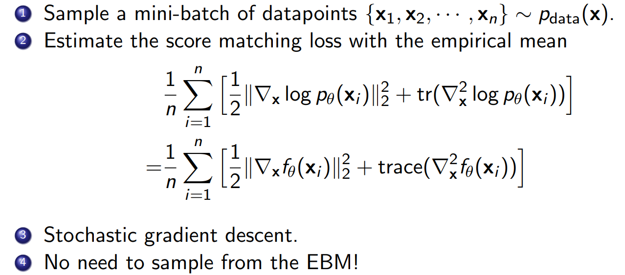
위 식을 활용한 score matching 학습은 다음과 같다.

위 식에서 더 이상 sampling이 필요하지 않은 것을 볼 수 있다. 그러나 위 식은 hessian 계산은 모델이 커질수록 연산이 많아진다는 단점을 갖는다.

Noise Contrative Estimation

Noise contrative estimation은 energy-based model을 noise distribution과 contrasting 하여 학습하는 방법이다. data distribution $p_{data}(\mathbf{x})$와 noise distribution $p_n(\mathbf{x})$ 를 contraisting 한다. 이때 noise distribution은 analytically tractable하고 sampling 하기 쉬은 distribution으로 설정한다.

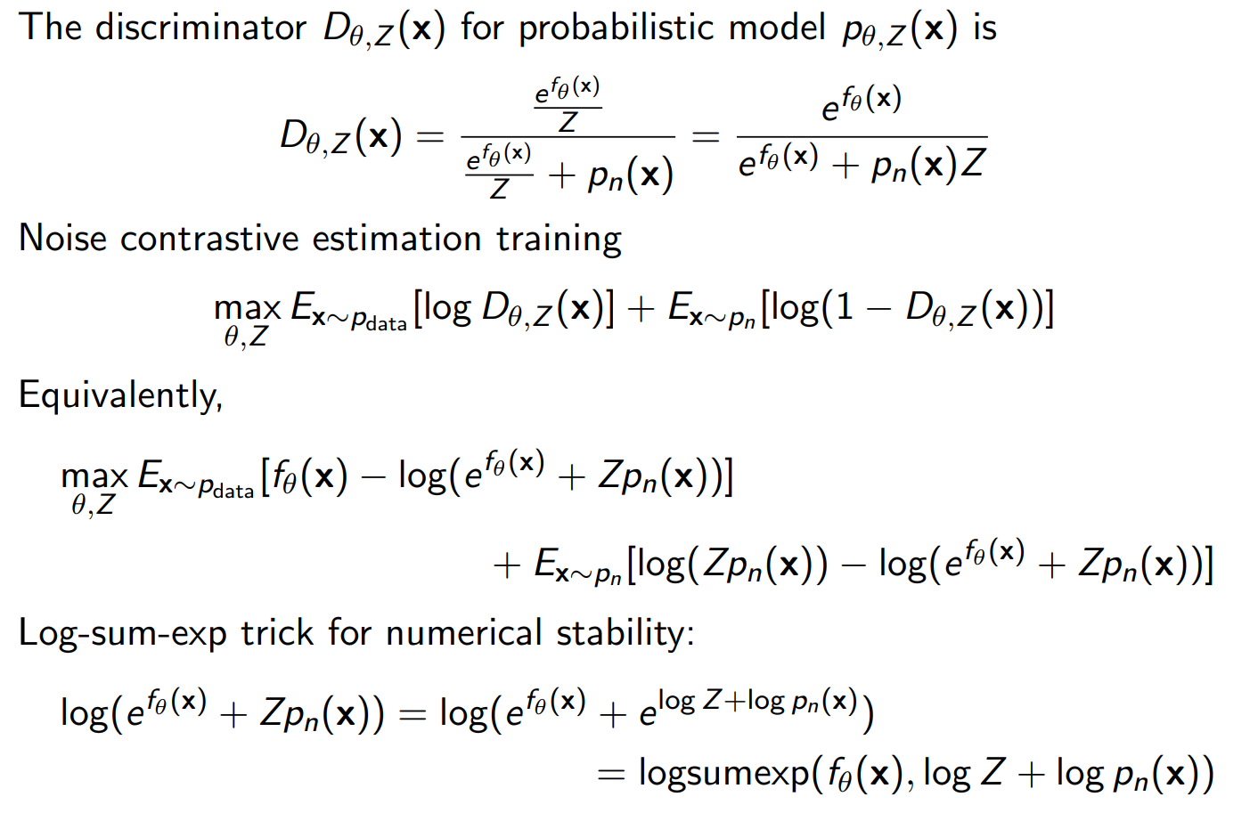
학습은 GAN과 유사하게 discriminator를 통해 학습을 진행한다. discriminator는 data samples와 noise samples를 구별한다.

• $\underset{\theta}{\max}E_{\mathbf{x}\sim p_{data}}E[\log D_\theta(\mathbf{x})]+E_{\mathbf{x}\sim p_n}[\log(1-D_\theta(\mathbf{x}))]$

위 식의 $D_\theta$는 다음과 같은 optimal 값을 갖는다.

• $D_{\theta^*}=\frac{p_{data}(\mathbf{x})}{p_{data}(\mathbf{x})+p_n(\mathbf{x})}$

만약 $D_\theta(\mathbf{x})=\frac{p_\theta(\mathbf{x})}{p_\theta(\mathbf{x})+p_n(\mathbf{x})}$로 설정하면 최적의 $D_\theta$는 다음과 같아진다.

• $D_{\theta^*}=\frac{p_\theta^*(\mathbf{x})}{p_\theta^*(\mathbf{x})+p_n(\mathbf{x})}=\frac{p_{data}(\mathbf{x})}{p_{data}(\mathbf{x})+p_n(\mathbf{x})}$

$p_\theta$를 energy-based model이라 하면 $p_\theta(\mathbf{x})=\frac{e^{f_\theta(\mathbf{x})}}{Z(\theta)}$가 된다. 이때 $Z(\theta)$는 $\int e^{f_\theta(\mathbf{x})}d\mathbf{x}$ 여야만 하는데, 이를 만족시키는 $Z(\theta)$를 찾기 어렵다. 이를 해결하기 위해 $\int e^{f_\theta(\mathbf{x})}d\mathbf{x}$ constraint를 만족하는 $Z(\theta)$를 찾는 것 대신 learnable parameter $Z$를 추가한다.

• $p_{\theta, Z}(\mathbf{x})=\frac{e^{f_\theta(\mathbf{x})}}{Z}$

위 식의 optimal parameter $\theta^*, Z^*$은 $p_{\theta^*,Z^*}(\mathbf{x})=p_{data}(\mathbf{x})$가 되어야한다. 따라서 $Z^*$는 기존의 partition function과 동일하다.

Noise Contrative Esitimation for Traning

Noise contrastive estimation의 학습 objective는 log-sum-exp trick을 이용해 다음과 같이 정리 될 수 있다.

그리고 objective function을 이용한 training 과정은 다음과 같다.

위 슬라이드에서도 알수 있듯이, 학습과정에서는 더 이상 sampling을 필요로 하지 않는다. 하지만 학습이 끝난 후에는 MCMC를 이용한 sampling을 해야한다.

Reference

cs236 Lecture 12