Score-based Models

지금까지 공부한 generative models의 벤 다이어 그램을 그리면 다음과 같은 관계를 볼 수 있다.

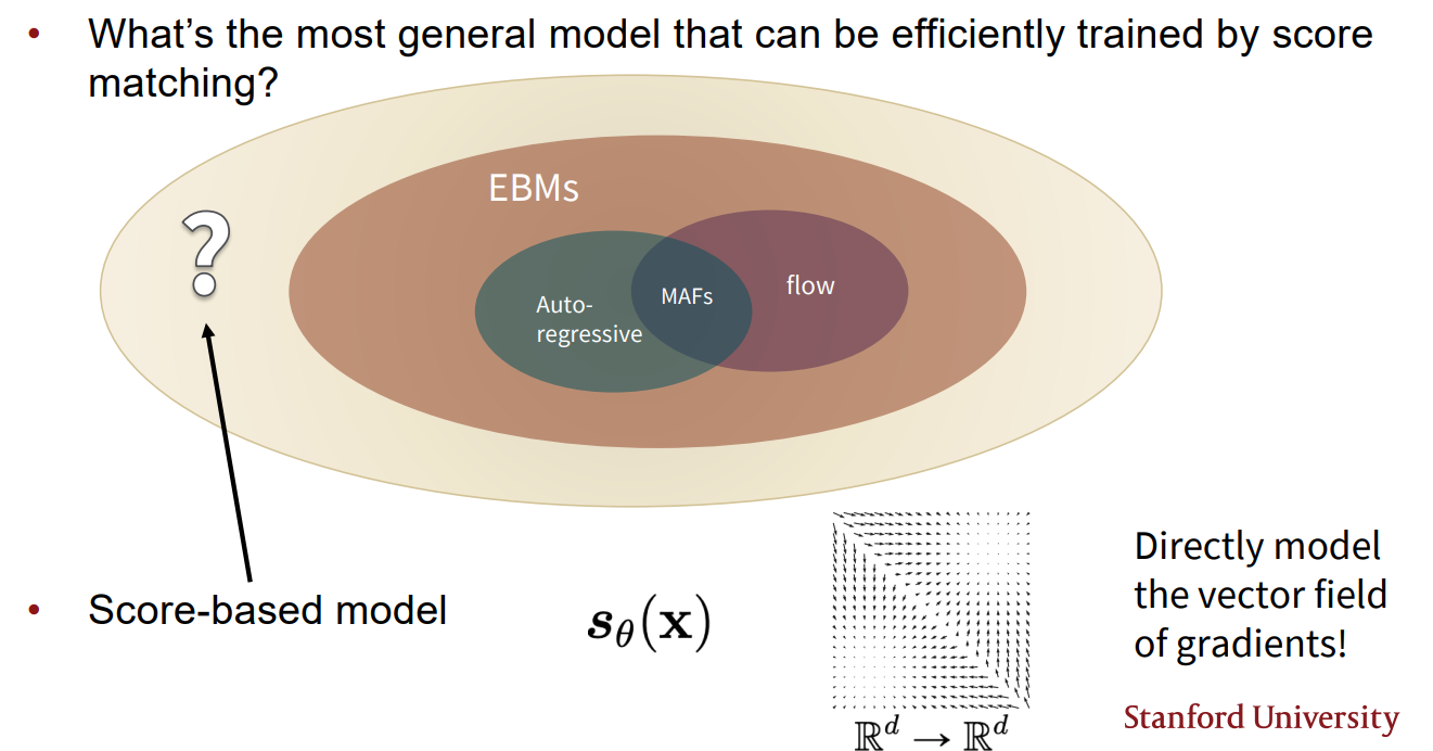
기존 Auto-regressive model과 Flow model이 likelihood를 바로 최적화 하여 modeling 하는 방식이었다면, Energe-based model에서는 partition function 문제를 해결하기 위해 pdf를 modeling하는 것인 아닌 score function 등을 modeling 하는 방식으로 generative models를 학습하였다. score-based models는 한 단계 더 나아가 score function 즉, gradients의 vector field를 직접 modeling 하는 generative model이다.

앞서 살펴본 Energy-based model을 score matching 방식으로 학습하는 것도 Score-based model의 일종이라 볼 수 있다. score matching은 score function을 estimation 할 때, objective로 두 vector filed의 Average Euclidean distance를 이용한 방식이다.(Fisher divergence)

Denoising Score Matching

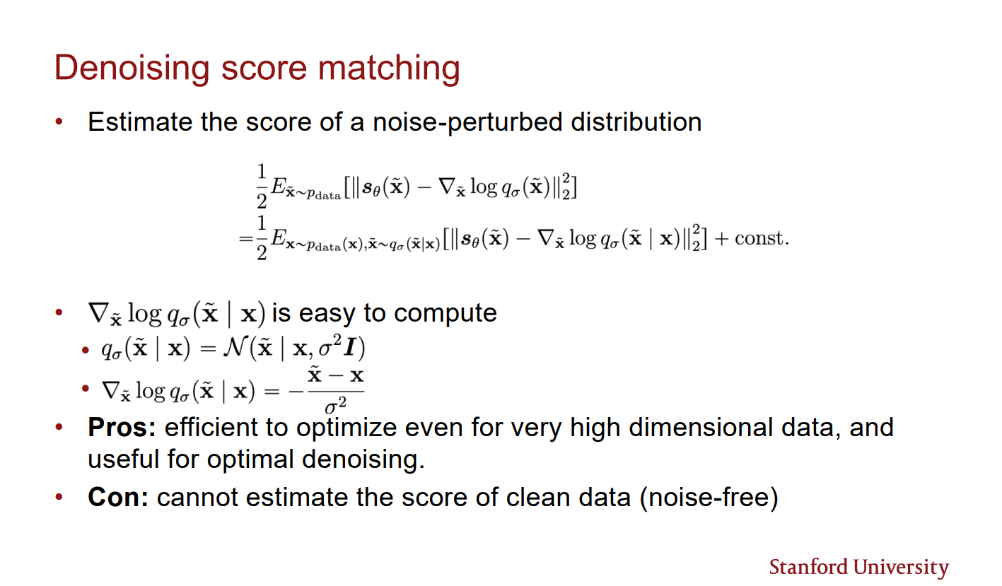
Score matching은 Euclide distnace를 이용하여 score function을 학습하는 방식이다. 그러나 score matching 방식은 scaleable 하지 않다. 왜냐하면 variable $\mathbf{x}$의 dimension $d$ 가 커질 수록 score function의 hessian 연산량이 커지기 때문이다.

이러한 문제를 Denosing score matching은 perturbed 된 $\mathbf{x}$를 이용하여 해결하였다.

• $q_\sigma(\tilde{\mathbf{x}|\mathbf{x})}=\mathcal{N}(\mathbf{x};\sigma^2,I),\ q_\sigma(\tilde{\mathbf{x}})=\int p(\mathbf{x})q_\sigma(\tilde{\mathbf{x}}|\mathbf{x})d\mathbf{x}$

perturbed 된 distribution은 gaussian distribution이기 때문에 score estimation이 훨씬 수월하다. $\nabla_{\mathbf{x}}\log p_{\mathrm{data}}(\mathbf{x})$ 대신 $\nabla_{\tilde{\mathbf{x}}}\log q_\sigma(\mathbf{\tilde{x})}$ 를 estimation 한다. 만약 perturbed 할 때의 noise level이 낮다면, $q_\sigma(\tilde{\mathbf{x}})\approx p(\tilde{\mathbf{x}})$ 가 좋은 approximation이 된다.

Denosing score matching의 nosie-perturbed distribution에 대한 score estimation은 다음과 같이 쓸 수 있다.(유도 과정 생략)

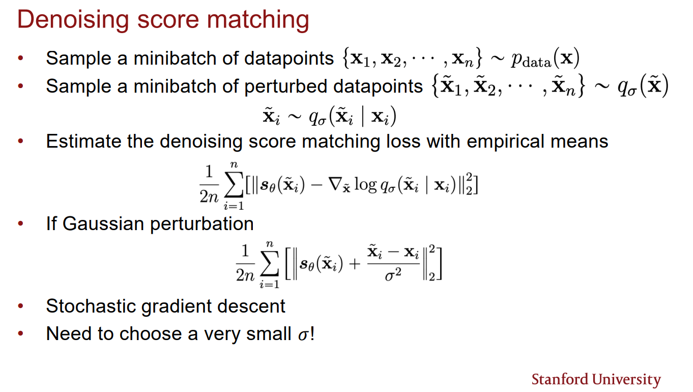
Denoising score matching 방식의 학습은 empiricla means를 이용하여 다음과 같이 이루어진다.

Denosing score matching은 score estimation이 비교적 쉽지만 noise가 끼지 않은 data에 대한 score estimation을 할 수 없다는 단점이 있다.

Tweedie's Formula

Denosing score mathcing의 학습 방식을 보면 nosing 된 distribution의 score를 matching 시키고 있을 뿐이다. 이는 왜 해당 방식이 denosing score mathcing이라 불리는지 이해하기 어렵다. Tweedie's formula는 이에 대한 해답을 준다.

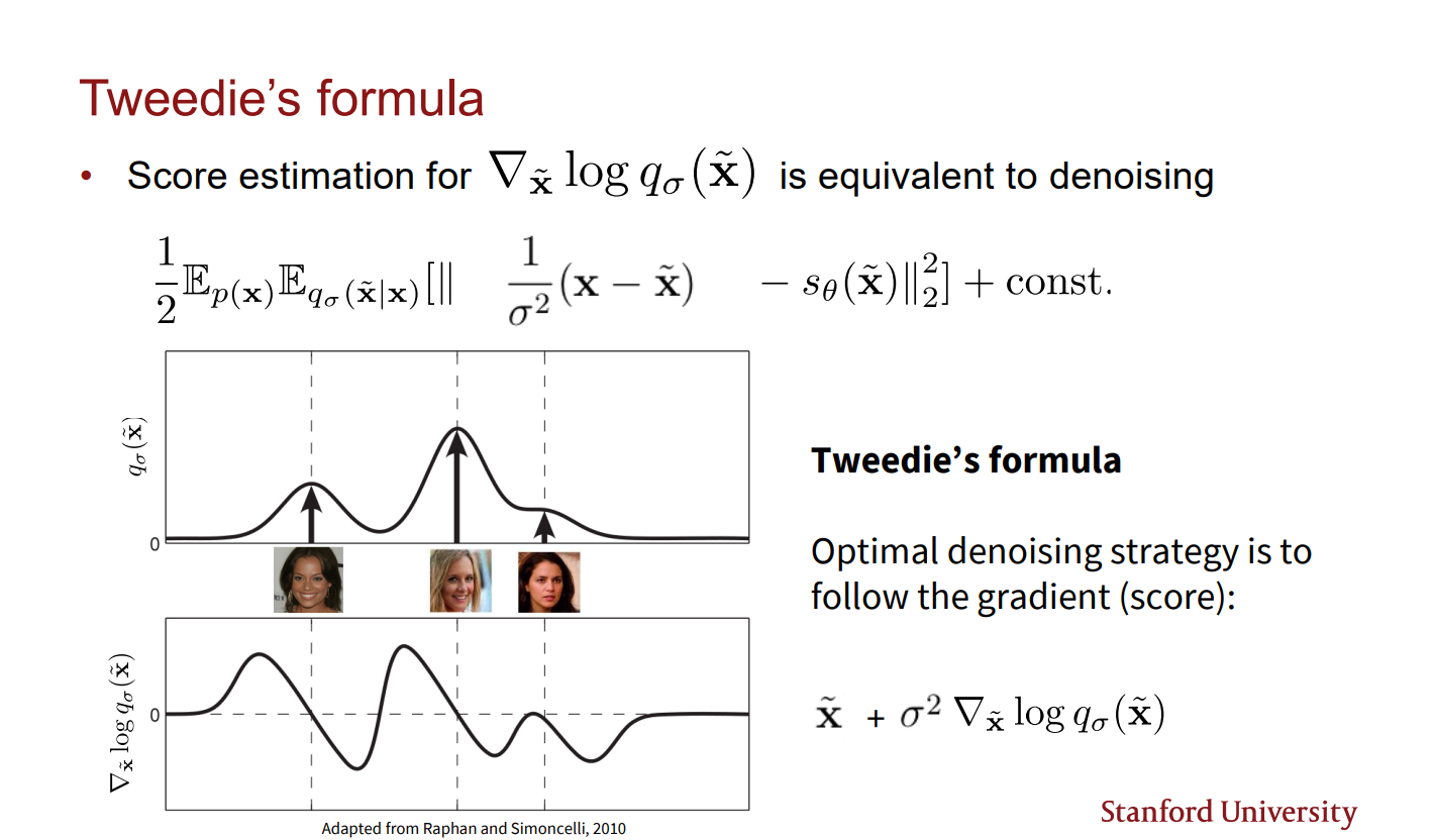
위 슬라이드르 보면 Denosing score matching 최적 전략은 데이터 포인트에 대한 gradient를 따라 가는 것임을 보여준다. 즉, $\tilde{\mathbf{x}}$ 에 대해 score function 방향으로 조정하면 최적의 denosing 결과를 얻을 수 있음을 알 수 있다.

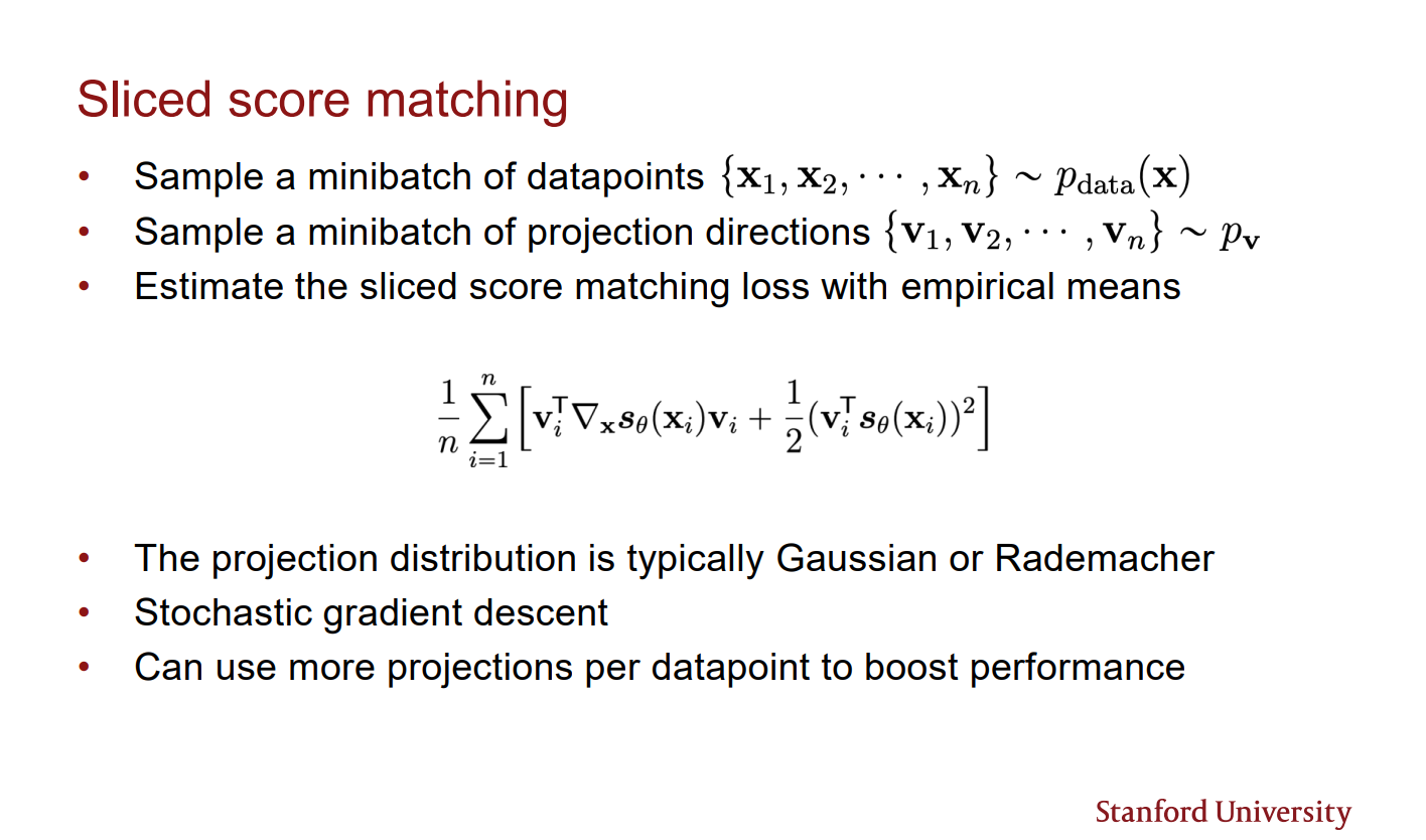
Sliced Score Matching

Scliced score matching은 어느 한 방향으로 gradient들을 projection 하여 matching 시키는 방식이다. obejctive는 다음과 같다.

• $\frac{1}{2}E_{\mathbf{v}\sim p_\mathbf{v}}E_{\mathbf{x}\sim p_{data}}[(\mathbf{v}^T\nabla_\mathbf{x}\log p_{data}(\mathbf{x})-\mathbf{v}^Ts_\theta(\mathbf{x}))^2]$
  이때 $\mathbf{v}$는 one dimensional random direction

부분 integration을 이용하면 다음과 같은 식으로 변형된다.

• $E_{\mathbf{v}\sim p_{\mathbf{v}}}E_{\mathbf{x}\sim p_{data}}[\mathbf{v}^T\nabla_\mathbf{x}s_\theta(\mathbf{x})\mathbf{v}+\frac{1}{2}(\mathbf{v}^Ts_\theta(\mathbf{x}))^2]$

$\mathbf{v}$가 one dimension 이기 때문에 jacobian 계산이 scalable 해진다.(jacobian 과 vector의 products는 scalar)

Sliced score matching의 학습 방식은 다음과 같다.

Score-based Model Sampling Pitfalls

Score-based model의 sampling 은 MCMC 방식을 이용하여 sampling 할 수 있다. 다음 MCMC의 일종인 Lagevin dynamics sampling 방식이다.

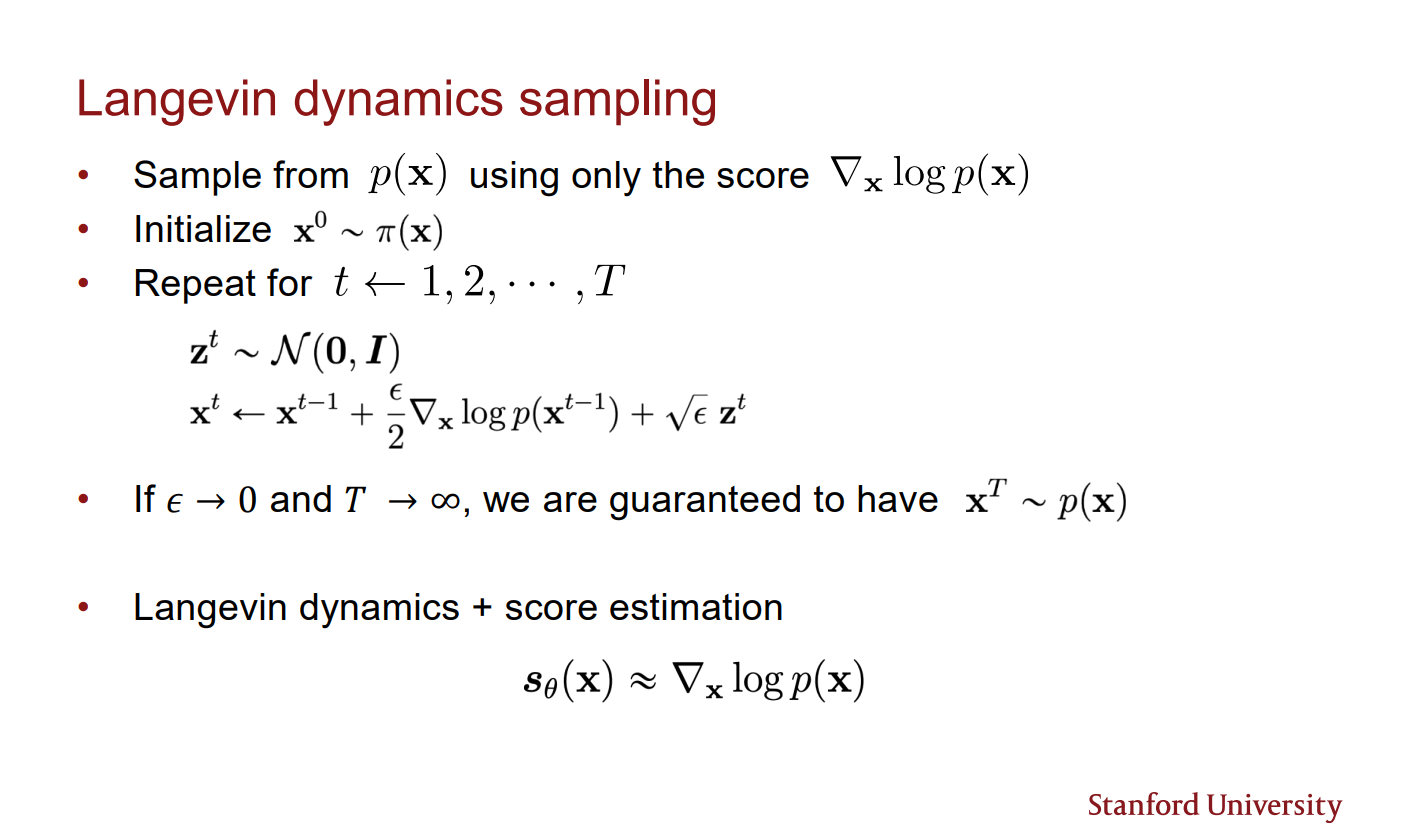
그러나 이러한 방식의 sampling은 좋은 결과를 얻지 못할 가능성이 크다. 그 이유는 다음과 같다.

1. 대부분의 data point는 manifold. 따라서 score가 정의되지 않음.
2. low data density 부분의 gradient estimation이 매우 부정확함. 따라서 해당 point에서의 sample을 올바르게 data distribution으로 수렴시키기 어려움
3. slow mixing of Langenvi dynamics between data modes. 2 개 이상의 mode(최빈값)가 있는 data distribution일 때 Lagevin dynamics는 두 mode 간의 이동이 매우 느림. 따라서 데이터 분포를 잘 표현하지 못할 수 있음.

Reference

cs236 Lecture 13