[Kaggle]집값 예측하기(House Prices prediction) - 2

KyeongHun Kim·2024년 1월 30일

ML/DL kaggle 데이터분석

ML/DL

목록 보기

4/8

지난 시간에는 Datset의 데이터를 확인했다. 계속 해보자!

📌 이전 글
[Kaggle]집값 예측하기(House Prices prediction) - 1

✍🏻 SalePrice Check

데이터 분포 재확인

예측 목표인 SalePrice의 분포를 확인했을 때 분포가 살짝 왼쪽으로 치우쳐있는 것을 확인했다. 이러한 경우 왜도와 첨도를 줄여 정규 분포의 형태로 만들어주는 것이 필요하다.

# log transform
train_df["SalePrice"] = np.log(train_df["SalePrice"]) # 값이 10만 단위이기 때문에 log변환을 진행

❓로그 변환(Log transform)

로그 변환이란 큰 수 x에 로그를 취해 작은 수로 만드는 것을 말한다. 분포가 치우쳐져 있을 때, 특히 왼쪽으로 치우쳐져 있을 때(Positive Skewness)일 때 사용하면 유용하다.

하지만, 데이터를 변경한 경우이기 때문에 해석에 주의해야 한다.

# 'SalePrice' 분포 시각화 및 QQ-Plot
sns.histplot(train_df['SalePrice'], kde = True, common_norm=True)

#Now plot the distribution
plt.legend(['Normal dist. ($\mu=$ {:.2f} and $\sigma=$ {:.2f} )'.format(mu, sigma)],
            loc='best')
plt.ylabel('Frequency')
plt.title('SalePrice distribution')

#Get also the QQ-plot -> SalePrice와 정규분포 비교
fig = plt.figure()
res = stats.probplot(train_df['SalePrice'], plot=plt)
plt.show()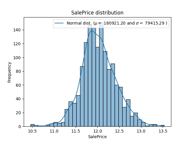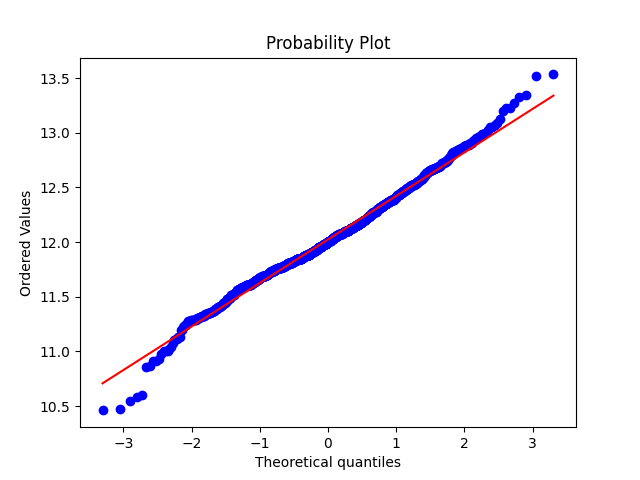

✍🏻 Check Selected Columns

SalePrice와 관련이 있다고 생각했던 Columns들을 확인해보자. 각각 'Neighborhood', 'OverallCond', 'YearBuilt', 'GrLivArea', 'TotalBsmtSF' 컬럼을 확인할 것이다.

# Scatter Plot SalePrice and selected column(Numeric data)
plt.figure(figsize = (20, 6))

plt.subplot(1, 3, 1)
plt.title("Scatter Plot SalePrice and YearBuilt")
plt.scatter(x=train_df['YearBuilt'], y=train_df['SalePrice'])

plt.subplot(1, 3, 2)
plt.title("Scatter Plot SalePrice and GrLivArea")
plt.scatter(x=train_df['GrLivArea'], y=train_df['SalePrice'])

plt.subplot(1, 3, 3)
plt.title("Scatter Plot SalePrice and TotalBsmtSF")
plt.scatter(x=train_df['TotalBsmtSF'], y=train_df['SalePrice'])

plt.show()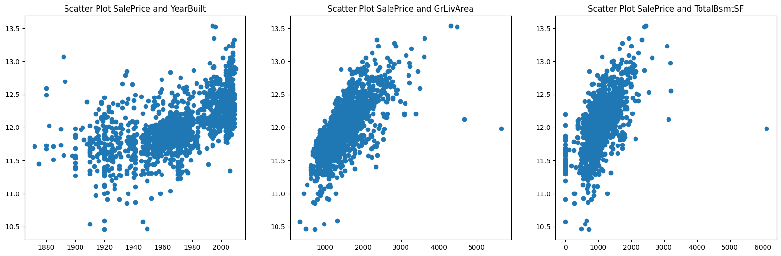

# boxplot
plt.figure(figsize = (12, 12))
sns.boxplot(x=train_df["SalePrice"], y=train_df['Neighborhood'], 
						palette="flare", hue = train_df["Neighborhood"], legend = False)
plt.title("SalePrice by Neighborhood")
plt.show()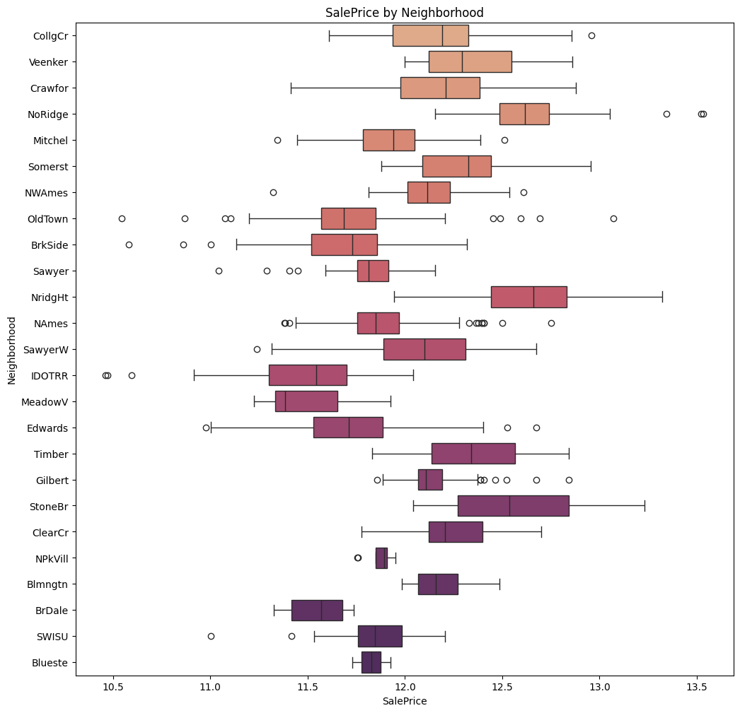

plt.figure(figsize = (12, 12))
sns.boxplot(x=train_df["OverallCond"], y=train_df["SalePrice"], 
						palette="flare", hue = train_df["OverallCond"], legend = False)
plt.title("SalePrice by OverallCond")
plt.show()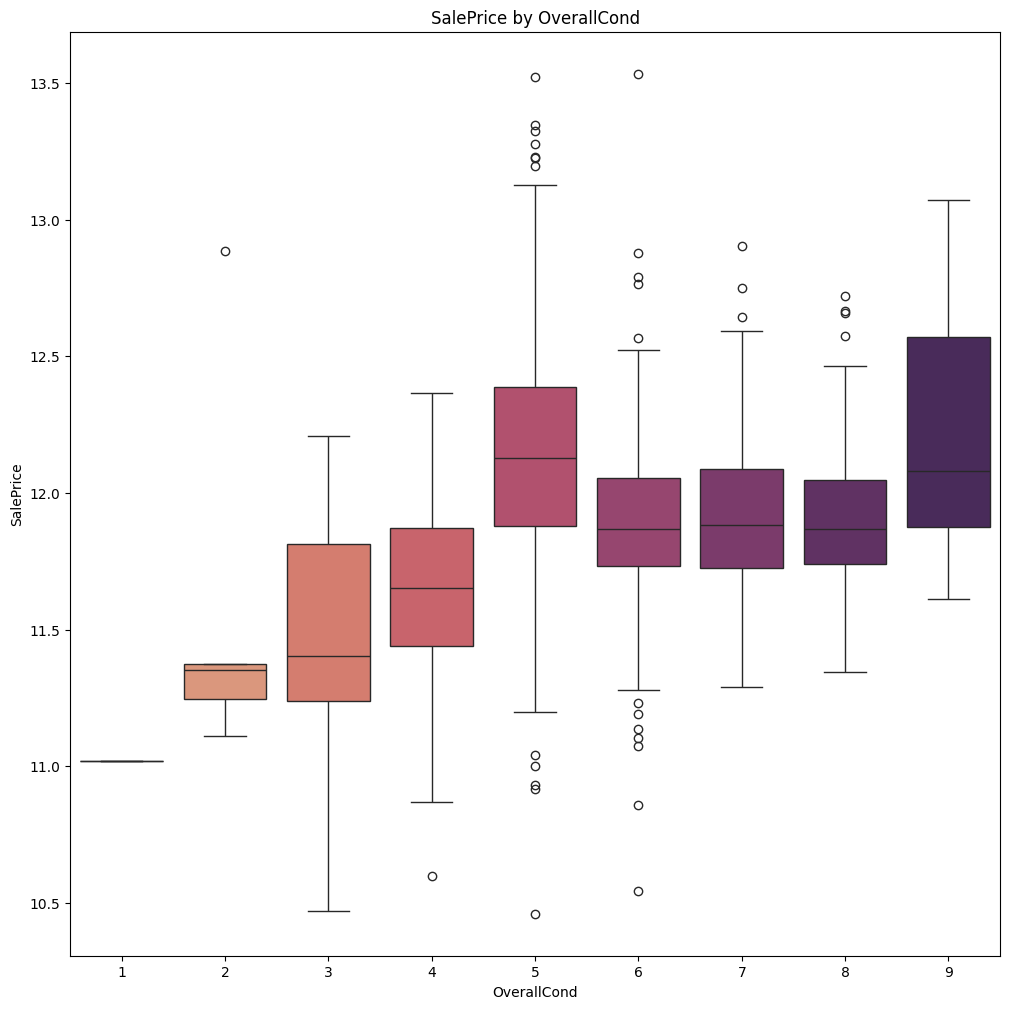

✍🏻 Feature Engineering

어떤 데이터를 처리할 때는 Test Dataset과 Train Dataset을 동일하게 처리해야 한다. 그러기 위해서 Test Data와 Train Data를 합쳐 All Dataset을 만든다.

train_num = train_df.shape[0]
test_num = test_df.shape[0]

all_dataset = pd.concat((train_df, test_df)).reset_index(drop=True)
all_dataset.drop(["SalePrice"], axis = 1, inplace = True) # Target Feature인 SalePrice는 제거

all_dataset.shape

> output (2919, 79)

결측치 확인 및 처리

데이터셋에서 NaN, None 등으로 표기되어 있는 곳들은 결측치이다. 이것들을 적절히 처리하지 않으면 학습에 영향을 줄 수 있기 때문에 처리해야 한다.

all_dataset_na = (all_dataset.isnull().sum() / len(all_dataset)) * 100 # Column별 결측치 비율 확인
all_dataset_na = all_dataset_na.drop(all_dataset_na[all_dataset_na == 0].index).sort_values(ascending = False) # 내림차순 정렬, 결측치가 없는 Column은 제외
missing_data = pd.DataFrame({"MissingRatio" : all_dataset_na})
missing_data

# 결측치 비율 확인
plt.figure(figsize = (12, 6))
sns.barplot(x = missing_data.index, y = missing_data["MissingRatio"],
			palette="flare", hue = missing_data.index, legend = False)
plt.title("Percentage of Mission Data by Feature")
plt.xticks(rotation = 90)
plt.xlabel("Features")
plt.ylabel("Percentage of Mission Data")
plt.show()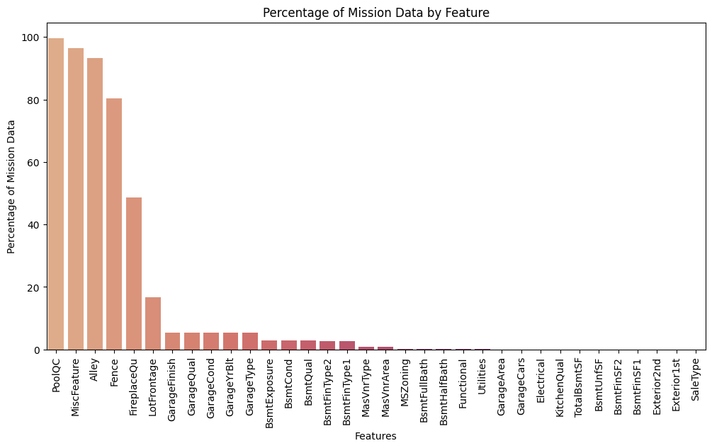

결측치를 처리하는 방법은 여러가지가 있으나 70% 이상의 결측치를 가지고 있는 Feature는 삭제, 0%에 가까운 결측치는 행을 삭제, 나머지 결측치는 'None' 값으로 대체한다.

# Delete Missing Ratio over 70%
drop_columns = list(missing_data.loc[missing_data["MissingRatio"] > 70].index)

all_dataset = all_dataset.drop(drop_columns, axis = 1)
all_dataset.shape

# Delete Missing data under 5%, 컬럼 삭제가 아닌 행 삭제
drop_columns = list(missing_data.loc[missing_data["MissingRatio"] < 5].index)

for column in drop_columns:
    index = all_dataset.loc[all_dataset[column].isnull()].index
    all_dataset = all_dataset.drop(index, axis = 0) # 행 삭제

# Impute Missing data
impute_columns = list(missing_data.loc[(missing_data["MissingRatio"] < 70) 
						& (missing_data["MissingRatio"] > 5)].index)

for column in impute_columns:
    if all_dataset[column].dtype == ('float64' or 'int64'): # 수치형 자료의 경우 0으로 채워넣기
        all_dataset[column].fillna(0, inplace = True)
    else: # 범주형 자료의 경우 'None'으로 채워넣기
        all_dataset[column].fillna('None', inplace = True)

Impute 과정에서의 문제점

결측치가 존재하는 column을 확인한 결과 특정 값을 넣어줄 필요가 있음을 파악함. 예를 들어 Garage와 관련된 column의 경우 'NA'(No Garage) 값을 넣어야 함.

# Impute Missing data
impute_columns = list(missing_data.loc[(missing_data["MissingRatio"] < 70) & (missing_data["MissingRatio"] > 5)].index)

# Grage data는 NaN 값을 'NA'로 처리
# FirePlaceQu는 NaN 값을 'TA'로 처리

for column in impute_columns:
    if column[:6] == 'Garage':
        all_dataset[column].fillna('NA', inplace = True)
    elif column[:4] == 'Fire':
        all_dataset[column].fillna('TA', inplace = True)
    else:
        all_dataset[column].fillna(0, inplace = True)

Encoding

학습을 위해 Categorical Data를 Encoding한다. 그 전에 범주형 자료이지만 숫자로 표기된 Column들은 str type으로 데이터를 변경시킨다. 이후 Pandas의 get_dummies() 메서드를 사용한다.

#MSSubClass=The building class
all_dataset['MSSubClass'] = all_dataset['MSSubClass'].apply(str)

#Changing OverallCond into a categorical variable
all_dataset['OverallCond'] = all_dataset['OverallCond'].astype(str)

#Year and month sold are transformed into categorical features.
all_dataset['YrSold'] = all_dataset['YrSold'].astype(str)
all_dataset['MoSold'] = all_dataset['MoSold'].astype(str)

cols = [column for column in all_dataset.columns if all_dataset[column].dtype == 'object'] # get_dummies 메서드에 사용할 Columns

all_dataset = pd.get_dummies(all_dataset, columns = cols, drop_first = True)
all_dataset.shape