[Mathematical Statistics] 2. Extension to several random variables

2.6 Extension to several random variables

다변수 확률 분포에서의 정의는 이변량 확률벡터를 다변량 벡터로 확장하기만 하면 된다. (단변량 vs. 다변량, 다변량일 경우 random vector 에 속함을 기억하자. 다변량 내에서도 bivariate r.v 가 조금 더 특수한 상황이고, 일반적으로 multivaritate 를 말한다면 이변량을 넘어서는 일반적인 다변량 확률벡터로 이해하자.)

Definition (Joint distribution). Let $d \in \mathbb{N}$. $\mathbf{X}:=\left(X_{1}, X_{2}, \ldots, X_{d}\right)^{T}$ is called a (multivariate) random vector ((다변량) 확률벡터) if $\mathbf{X}(\cdot)$ is a multivariate function that maps $c \in \mathcal{C}$ to $\mathbf{X}(c):=\left(X_{1}(c), X_{2}(c), \ldots, X_{d}(c)\right) \in \mathbb{R}^{d}$, i.e., $\mathbf{X}: \mathcal{C} \rightarrow \mathbb{R}^{d}{ }^{1}{ }^{1}$

조금 더 간단한 정의는 다음과 같다.

An equivalent definition is that $\mathbf{X}$ is a random vector if each component of $\mathbf{X}$ is a random variable.

각 random variable 을 모은 random vector 라 보고 넘어가자.

vector X에 대한 notation 과 space of X는 다음과 같다.

• We will use the vector notation $\mathbf{X}=\left[\begin{array}{c}X_{1} \\ X_{2} \\ \vdots \\ X_{d}\end{array}\right]=\left(X_{1}, X_{2}, \ldots, X_{d}\right)^{T}$,

• The space of $\mathbf{X}$ is $\mathcal{D}=\left\{\mathbf{x} \in \mathbb{R}^{d}: x_{1}=X_{1}(c), x_{2}=X_{2}(c), \ldots, x_{d}=\right.$ $\left.X_{d}(c), c \in \mathcal{C}\right\}$.

다변량 확률벡터에 대해서도 joint cdf 와 joint pmf, joint pdf 를 정의하는 것이 가능하다. 이미 익숙한 내용이지만 차이점을 중심으로 눈여겨 보자.

• The joint cdf (결합누적분포함수) of $\mathbf{X}$ is defined by

joint cdf 는 각 확률변수가 주어진 값보다 각기 작거나 같은 확률을 and 로 연결한 것이다.

• A random vector $\mathbf{X}$ is called discrete if there exists a countable subset $S \subseteq \mathbb{R}^{d}$ such that $P\left(\mathbf{X} \in S^{c}\right)=0$. For a discrete r.v. $\mathbf{X}$, the joint pmf (결합확률질량함수) is defined by

pmf 는 X 가 discrete 일 경우 각 확률변수가 주어진 값을 가질 확률로 정의하면 된다. discrete 이고 정의부터 그 외의 subset 에 대해선 확률이 0인 것을 감안하면, $S_{\mathbf{X}}=\operatorname{supp}(\mathbf{X}):=\left\{\mathbf{x} \in \mathbb{R}^{d}: p_{\mathbf{X}}(\mathbf{x})>\right.$ $0\}$ 임이 자연스럽다.

• 마지막으로 X가 continuous 일 경우에 어떠한 nonnegative function g가 다음을 만족시킨다면 (non-negative function 의 적분으로 정의되는 cdf가 있다면) 그 g는 joint pdf이며, $f_{\mathbf{X}}(\mathrm{x})$. 와 같이 적는다.

(다음이 존재; 어떤 함수를 x1, x2, ...xd까지 적분하여 joint cdf가 되는 nonnegative function 존재.)

($f_{\mathbf{X}}(\mathrm{x})$.➡️ 각 확률변수가 취하는 small x에 대해 d번 편미분)

expected value of Y (변환의 기댓값)은 다음과 같다.

변환의 기댓값은 이변량/단변량을 다변량으로 확장시킨 것 외에 같은 form 으로 이해 가능하다. 만약 헷갈린다면.. 1.8절로 돌아갔다 오자.✅

mgf 는 그냥 X 대신에 random vector X가 들어가며 이 역시 나머지는 같다.

• mgf. Let $X_{1}, \ldots, X_{d}$ be random variables and suppose that $\mathrm{E}\left\{\exp \left(t_{1} X_{1}+\right.\right.$ $\left.\left.\cdots+t_{d} X_{d}\right)\right\}$ exists for $-h_{i}<t_{i}<h_{i}$ for some $h_{i}>0(i=1, \ldots, n)$. Then the moment generating function (mgf) of the joint distribution of the random variables is

2.7 Transformation of random vectors

random vector X에서 Y로의 변환에 대해 알아보도록 하자.

Consider transforming $d$ random variables $X_{1}, \cdots, X_{d}$ to $d$ random variables $Y_{1}, \cdots, Y_{d}$ s.t. $y_{1}=u_{1}\left(x_{1}, \cdots, x_{d}\right), \cdots, y_{d}=u_{d}\left(x_{1}, \cdots, x_{d}\right)$.

2.7.1 One-to-one transformation case
여기서는 랜덤벡터의 변환을 one-to-one 인 경우와, many-to-one 인 경우 두 가지로 나누어서 구할 것이다. 먼저 X와 Y의 1-1 경우에 대해 알아보자. Y의 표현은 다음과 같이한다. 이 경우 랜덤벡터가 어떻게 구성되는 지 확인할 수 있다.

변환에서 중요한 것은 pdf of Y를 pdf of X와 Jacobian 을 가지고 쓸 수 있다는 것이었다. 다음은 pdf of Y를 구하는 방법.

• $\mathbf{w}=\left(w_{1}, \ldots, w_{d}\right):=\mathbf{u}^{-1}$ 는 X에서 Y의 변환인 u의 inverse transformation 이다.
• $J=\partial \mathbf{x} / \partial \mathbf{y} \in$ $\mathbb{R}^{d \times d}$ be the Jacobian of the transformation $\mathbf{x}=\mathbf{w}(\mathbf{y})$. -> x를 y로 편미분 한 것의
• determiannt 를 곱해주면 됨.

(Example)
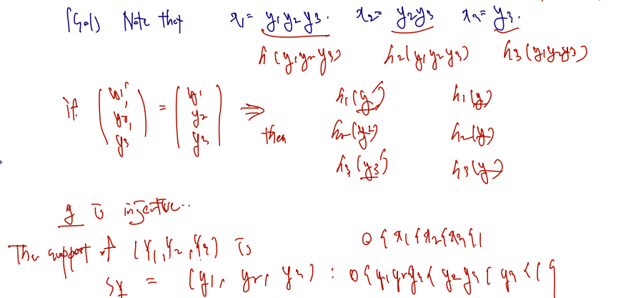
Let $\mathbf{X}=\left(X_{1}, X_{2}, X_{3}\right)^{T}$ have the joint pdf $f\left(x_{1}, x_{2}, x_{3}\right)=48 x_{1} x_{2} x_{3}$, $0<x_{1}<x_{2}<x_{3}<1$. Let $Y_{1}=X_{1} / X_{2}, Y_{2}=X_{2} / X_{3}$ and $Y_{3}=X_{3}$

• Find the joint pdf of $\left(Y_{1}, Y_{2}, Y_{3}\right)$.

• X에서 Y로의 변환이 g라고 할 때, g가 injective 임을 보인다.
• 주어진 x1, 2, 3 사이의 부등식을 이용해 support of Y를 새롭게 쓴다.

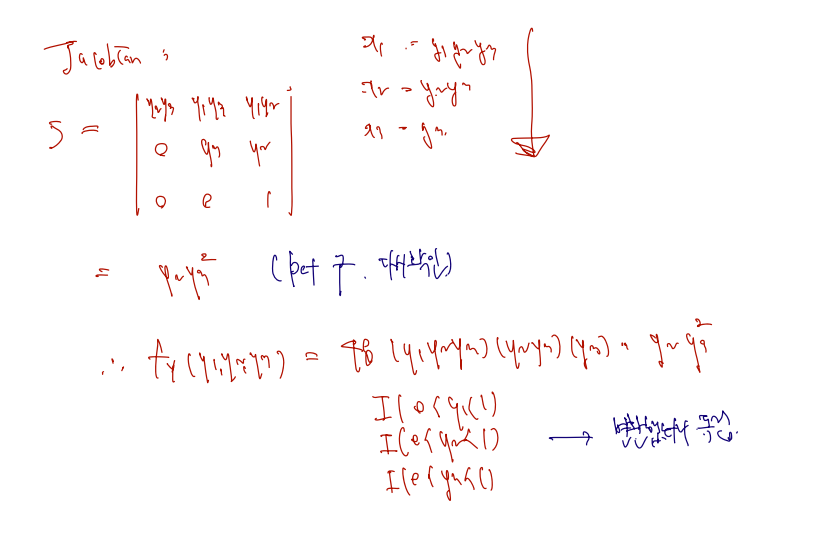
• Jacobian 을 쓰고 determiant 를 구하는데, 변수를 헷갈리지만 않으면 어렵지 않게 구할 수 있다.
• pdf of X와 Jacobian 의 곱의 형태로 pdf of Y를 완성한다. Support of Y를 다시 써주면 완성.
• 이 문제에서처럼 변환 전에는 그렇지 않았던 변수가 변환 후 독립성이 확인되는 경우가 있을 수 있다.

2.7.2 Many-to-one transformation case

many-to-one 의 정의는 다음과 같다.

Definition. (many-to-one transformation case)
A map $\mathbf{u}: \mathcal{X} \rightarrow \mathcal{Y}$ is called $k-1$ ( $k$ to one), if there exist $A_{1}, \cdots, A_{k}$ such that $\bigcup_{i=1}^{k} A_{i}=\mathcal{X}$ and $A_{i} \cap A_{j}=\phi$ for $i \neq j$ (i.e., $A_{1}, \cdots, A_{k}$ exhaustive sets), and $A_{i} \xrightarrow{\mathbf{u}} \mathcal{Y}$ is injective for each $i=1, \cdots, k$.

• 집합 A의 각각의 합집함이 X가 되고, 어떤 임의의 i, j에 대해서도 겹치지 않을 때 (다시 말해 X의 사상을 1-1로 뜯을 때)
• 각 A에 대해 Y로의 1-1 transformation 을 만족하면 된다.

(many-to-one 의 pdf 표현에 대해선 충분히 이해하지 못했다. 다시 이해한 후 설명을 추가할 예정)

2.8 Linear combinations of random variables

rancom variables (vectors)에 linear 변환을 한 것의 expetation, covariance, variance에 관심을 기울이자.

먼저 Let $X_{1}, \ldots, X_{n}$ be r.v.s and define $T=\sum_{i=1}^{n} a_{i} X_{i}$ for some constants $a_{1}, \ldots, a_{n}$. 라 하자. 이는 기존에 우리가 알던 변수 X에 대해 단순히 $a_{i}$ 가 곱해진 형태이며, 아래와 같은 주장들이 가능해진다.

1. 기댓값) Then, $E(T)=\sum_{i=1}^{n} a_{i} E\left(X_{i}\right)$.

• linearity of expectation

2. 공분산) 또다른 W를 같은 Y에 대해 $b_{i}$ 가 곱해진 변수로 이해할 때,
   Let $X_{1}, \ldots, X_{n}, Y_{1}, \ldots, Y_{m}$ be r.v.s and define $T=\sum_{i=1}^{n} a_{i} X_{i}$ and $W=\sum_{j=1}^{m} b_{j} Y_{j}$ for some constants $a_{1}, \ldots, a_{n}, b_{1}, \ldots, b_{m}$. If $E\left(X_{i}^{2}\right)<\infty$ and $E\left(Y_{j}^{2}\right)<\infty$ for $i=1, \ldots, n$ and $j=1, \ldots, m$, then

• bi-linearity

3. 분산) Let $X_{1}, \ldots, X_{n}$ be r.v.s and define $T=\sum_{i=1}^{n} a_{i} X_{i}$. If $E\left(X_{i}^{2}\right)<$ $\infty$ for $i=1, \ldots, n$, then

4. 독립조건 가) 여기에 독립 조건이 추가된다면 Let $X_{1}, \ldots, X_{n}$ be independent r.v.s and define $T=\sum_{i=1}^{n} a_{i} X_{i}$. Then,

사실은 이 주장들은 covariance matrix 를 시각적으로 떠올려보거나 chapter 2.5의 properties of covariance 내용을 쓰면 수식으로 쉽게 쓸 수 있는 내용이다. 처음이라 생송할 수 있지만.. 이러한 곱의 형태나 linearity 를 이용해 쪼개는 것에 익숙해지면 보다 쉽게 covariance 를 이해할 수 있을 것으로 느껴진다. 일단 부단히 써보는 것.. 중요.