이 절에서는 최대 가능도 방법을 recall 하고 이전보다 더 다양한 mle 찾기에 대해 논의할 것이다. 먼저 MLE 최대 가능도 추정이 무엇이었는지 recall 하자.
Recall. Let X1,…,Xn be r.s. from a distribution with pdf1f(x;θ)(θ∈Ω⊂R.) Also, let X=(X1,…,Xn)T and x=(x1,…,xn)T represent the whole sample and its realization.
여기서 가정하는 상황은 모수 공간에서 모수가 1개인 경우다. (분포를 지배하는 모수가 여러개인 경우가 더 많으나 여기선 하나라고만 제한했다.) 세타를 true parameter 로 하는 pdf 에서 iid로 뽑은 random sample 이 있다고 하자. 이들의 뽑은 후 값은 realization 이라고 하였고, 이를 바탕으로 아래 함수들이 정의되었다.
(추가🤔)
나중에 다시 다룰 기회가 있을지 모르지만, 어떤 분포를 다루는 모수가 존재하고 이 pdf 에서 sample 들이 나왔다고 하는 건 매우 강한 가정이다. 왜냐? 현실세계에선 데이터를 얻어도 이 데이터들이 어떤 분포를 따르는지 단박에 알기 어렵고 사실상 "all models wrong, some are useful" 의 의미를 따라야하기 때문이다. 그러나, 어떤 알고 있는 pdf 를 가정할 경우, 그 모수를 추정하는 여러 추정량, 추정 방법 중 MLE 는 매우 강력한 도구이다. 그 이유도 이 포스트에서 다룰 것이다.
가능도 함수는 주어진 true parameter theta에서 표본이 추출되었을 때, 각 x1...xn 표본을 관찰할 확률을 theta에 대해 표시한 것이다. 예컨대 true paramter 가 아닌 다른 세타값을 넣으면 (다른 세타값을 넣는다는 것은 그 세타를 가정했을 때 표본의 관찰할 확률을 계산하는 것과 같다.), true parameter 와 비교해 가능도함수 값이 떨어질 것이다.
Maximum likelihood estimator (최대가능도추정량) of the true parameter θ given sample X :
θMLE:=θ∈ΩargmaxL(θ;X)=θ∈Ωargmaxl(θ;X).
우리가 궁금한 것은 항상 데이터가 주어졌을 때 이들이 따르는 분포, 분포의 모수가 무엇인지 값으로 밝혀내는 것이었다. 다른 말로 true parameter 와 근접하도록 이들을 추정하는 추정량을 계산해야 하고, by definition 에 따라 가능도 함수를 최대화하는 최대화원 세타를 MLE 추정량이라 한다. 왜냐? 가능도함수는 서로 다른 세타에 대해 그 관찰 확률을 값으로 계산하는데.. 그 값이 최대가 된다는 건 추정한 세타가 true parameter 에 가까워졌다는 뜻이기 때문이다.
이 절에서 보이고 싶은 것들을 증명하기 위해 아래의 theorem 이 필요하다. Theorem Assume that θ0 is the true parameter and that Eθ0[f(X1;θ)/f(X1;θ0)] exists. Under R0 and RI,
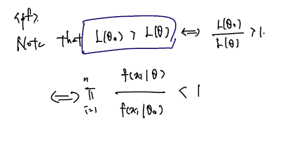
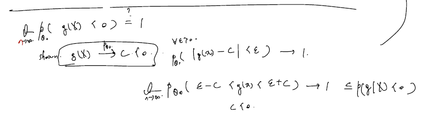
n→∞limPθ0[L(θ0;X)>L(θ;X)]=1, for all θ=θ0
직관적으로 해석 가능한 정리로, θ0 denote the true value of θ 라 했을 때 서로 다른 세타 사이에서 true theta 가 주어질 때 데이터를 관측할 확률이 이와 다른 세타가 주어질 때 확률보다 크다는 것, 클 확률이 n이 커질수록 1이라는 것이다. 이를 증명하기 위해 다음의 정칙성명하기 위해 다음의 정칙성 조건이 필요하다. (복잡하게보단 가볍게 알아두자.)
Assumption (Regularity Conditions). Regularity conditions (RO)-(R2) are (R0) The cdfs are distinct; i.e., θ=θ′⇒F(⋅;θ)=F(⋅;θ′)., 모수가 다르면 cdf 에서 값이 달라지는 x가 무조건 존재한다. 역으로, cdf 가 어떤 점 x에서 값이 다르다면 모수가 다르다. (counter example; N(μ+ϵ,1) 일 때 (\mu, epsilon) 이 각각 0 + 0 인 경우와 -1+1 인 경우.
(R1) The pdfs have common support for all θ., X의 supprot 는 theta에 depend 하진 않는다. (counter example; U(0,θ) 인 경우)
(R2) The point θ0 is an interior point in Ω.,d차원 real 에 존재한다. 경계에 있지 않다.
다시 theorem 을 증명해보자.
[1]
[2]
[보충]
Example 1 (Exponential distribution)
Example (Exponential distribution). Let X1,⋯Xn be r.s. from Exp(θ) with θ>0, i.e.
Since l′(θ)>0 for θ<Xˉ and l′(θ)<0 for θ>Xˉ (check!), θ=Xˉ is the MLE of θ.
한 번 미분해서 0이 되는 점은 표본평균이고, 표본평균을 기준으로 세타가 왼쪽 또는 오른쪽에 있을 경우에 증감을 따져볼 순 있으나.. 아래처럼 아예 치환을 하면 두 번 미분하기 좋을 것이다.
(sol2) Let η=1/θ and q(η)=l(1/η). Since η=1/θ is a bijective mapping on R+ to R+, the maximization of q(η) is equivalent to the maximization of l(θ). Then,
q(η)=q′(η)=q′′(η)=nlogη−η∑xiηn−∑xi(∴q′(η)=0⇒η=1/xˉ)−η2n<0 for all η>0
Thus, q(η) is uniquely maximized at η=1/xˉ and so l(θ) is uniquely maximized at θ=1/η=xˉ.∴θMLE=Xˉ.
두 번 미분했더니 모든 에타 점에서 0보다 작으므로 위로 한 번 미분 =0 지점이 위로 볼록의 MLE 였음을 확실히 보일 수 있다. (uniquely maximied at sample mean)
Example 2 (doest not have closed form solution)
Example (Logistic distribution). Let X1,⋯Xn be r.s. from pdf
f(x;θ)=(1+e−(x−θ))2e−(x−θ),−∞<x<∞,−∞<θ<∞
Find the MLE of θ.
(sol)
l(θ)l′(θ)l′′(θ)=nθ−i=1∑nxi−2i=1∑nlog{1+e−(xi−θ)}=n−2i∑{1+e−(xi−θ)}e−(xi−θ)=−2i∑{1+e−(xi−θ)}2e−(xi−θ)<0 for all θ
한 번 미분, 두 번 미분해서 모든 세타에 대해 0보다 작은 위로볼록인 함수임이 드러났으나 한 번 미분 = 0 인 점이 계산이 되지 않는다. 그렇다면 MLE 의 unique solution 이 없는걸까? 그렇지 않다. l′′(θ)<0 for all θ∈R,limθ→−∞l′(θ)=∞ and limθ→∞l′(θ)=−∞ 이므로
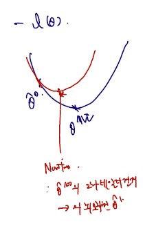
MLE 해가 존재하고, 유일성을 지니나.. closed form 으로 적을 수 없는 case 에 속한다. 이 경우 아래의 Newton's method 를 써볼 수 있다. (2차테일러 전개)
θ(t+1)←θ(t)−l′(θ(t))/l′′(θ(t))
첫 세타0에서 다음 세타1로 나아가기 위해 세타0에서 2차 테일러 전개한 후, 새로 쓴 함수에서 최소화원 세타1을 계산한다.
이 방법을 반복적으로 하는 것을 세타를 update 한다고 하며, 최소화원을 찾는 방법 중 하나에 속한다.
테일러 전개를 쓰는 이유는 테일러 전개가 곧 계산하고 싶은 (목표) 점의 위치를 (알고 있는) 다른 점의 위치, 1, 2차 미분으로 근사할 수 있다는 것이므로 motivation 이 같다.
Example 3 (prameter θ 가 Xi 에 depend 하는 경우)
Example (Uniform distribution). Let X1,⋯Xn be r.s. from U[0,θ], i.e,
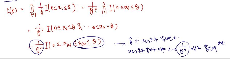
f(x;θ)=θ1I(0≤x≤θ),θ>0
Find the MLE of θ.
Xn은 sample X의 n번째 순서통계량
따라서 추정량 세타가 Xn 보다 작은 구간이 생기면 여기서 가능도함수 값이 0이니까 안되고..
그렇다면 Xn 보다 같거나 커야 하는데 커질수록 decay 하는 형태이므로 정확히 같은 점에서 Likelihood 값이 최대가 됨.
따라서 표본의 최댓값이 MLE
Example 4 (알려진 지식으로 parameter space 제한)
Example (Bernoulli distribution with restricted parameter space). Let X1,⋯Xn be r.s. from B(1,θ) with 0≤θ≤31. Find the MLE of θ.
(sol)
L(θ)=θ∑i=1nxi(1−θ)n−∑i=1nxi=θnxˉ(1−θ)n−nxˉ
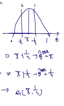
case1) If xˉ=0, 대입, then L(θ)=(1−θ)n 이므로 0=min{xˉ,1/3}, 0일 때 최대.
case2) if xˉ=1, 대입, then L(θ)=θn is maximized at 1/3=min{xˉ,1/3}.
case3) Now, assume that xˉ∈(0,1). 이때는 cancel 이 없으므로 함수 써야 함. 범위는 0<θ≤1/3. So,
l(θ)l′(θ)l′′(θ)=nxˉlogθ+(n−nxˉ)log(1−θ)=nθxˉ−n1−θ1−xˉ=−nθ2xˉ−n(1−θ)21−xˉ<0 for all θ
또는 그려볼 수 있음.
표본평균 < 1/3 인 경우, MLE 는 표본평균.
표본평균 > 1/3 인 경우, MLE 는 1/3
min(표본평균, 1/3) 으로 정리
Thus, θMLE=min{Xˉ,31}
위에 다룬 예제들과 별개로 앞으로 사용할 MLE 에 관련한 정리들을 증명 없이 간단히 살펴보자.
(MLE functional invariance) Theorem Let X1,…,Xn be iid with the pdf f(x;θ),θ∈Ω. For a specified function g, let η=g(θ) be a parameter of interest. Suppose θ is the MLE of θ. Then g(θ) is the MLE of η=g(θ). i.e., g(θ)MLE=g(θMLE).
만약 θ is the MLE of θ 라는 것이 이미 밝혀졌음에도 궁금하고 θ 이외에도 이를 변환한 다른 모수 η=g(θ) 도 추정하고 싶다고 하자. 그렇다면, 다른 계산 없이 이미 밝혀둔 θ 를 변환 g에 집어넣은 g(θ) 값이 η=g(θ)에 대한 MLE 라는 것이다.
Example. Let X1,⋯Xn be r.s. from B(1,θ),θ∈(0,1). Then we know that θMLE=Xˉ. So the MLE of θ(1−θ), the variance of B(1,θ), is θMLE(1−θMLE)=Xˉ(1−Xˉ)
binomial 의 모수 세타의 MLE 가 표본평균이란 건 이미 알려진 사실이라고 할 때,
이번엔 같은 모수 세타에 depend 하는 모분산이 궁금하다고 하면..
모분산으로 넘어가는 변환 g를 표본평균에 대해 적용하면 그것이 모분산의 MLE 가 된다.
(MLE Consistency)
Theorem 6.1.3. Assume that X1,…,Xn satisfy the regularity conditions R0 through R2, where θ0 is the true parameter, and further that f(x;θ) is differentiable with
respect to θ in Ω. Then we have a solution θn such that θnPθ0.
true parameter 가 interior 에 존재하고
pdf of x가 세타에 대해 미분가능하다면
가능도함수에 대해 MLE 가 여럿이 존재하는 경우 그 중 true parameter 로 in probability 수렴하는 MLE 는 하나 존재한다는 것이다.
다시말해, MLE 가 여러개라면 그 중 하나가 ture parameter 의 일치추정량이라는 것이다.
Corollary Assume that X1,…,Xn satisfy the regularity conditions R0 through R2, where θ0 is the true parameter, and that f(x;θ) is differentiable with respect to θ in Ω. Suppose the likelihood equation has the unique solution θn. Then θn is a consistent estimator of θ0.
따라서 만약 가능도함수가 유일한 최대화원을 가진다면 그 최대화원이 true parameter 의 일치추정량이라는 것이다.