AI_Tech부스트캠프 week13...[4] FCN 한계를 극복한 model1

Leejaegun·2024년 11월 11일

AI_tech_CV트랙 여정

목록 보기

40/74

1. FCN의 한계점

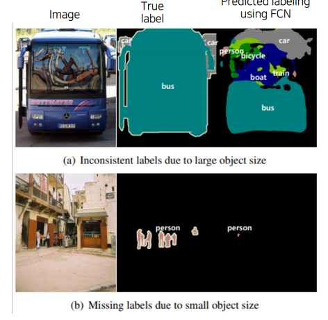
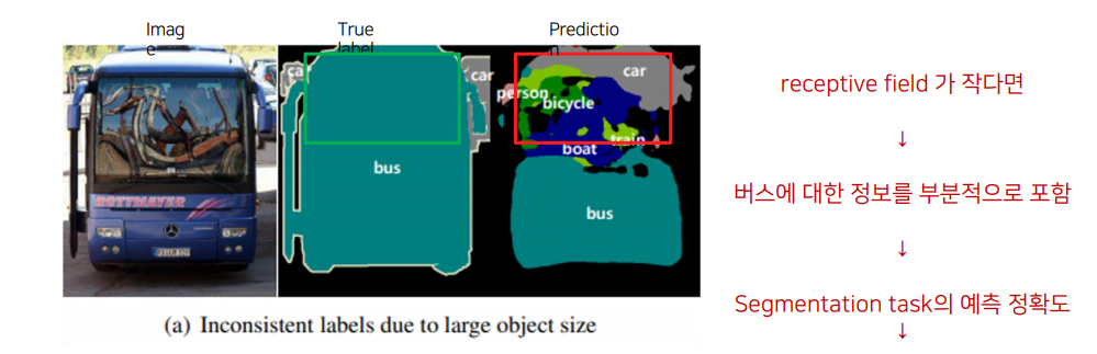
(1).객체의 크기가 크거나 작은 경우 예측을 잘 하지 못하는 문제

• 큰 Object의 경우 지역적인 정보만으로 예측
• 버스의 앞 부분 범퍼는 버스로 예측하지만, 유리창에 비친 자전거를 보고 자전거로 인식하는 문제 발생하기도 함
• 같은 Object여도 다르게 labeling
• 작은 Object가 무시되는 문제가 있음

(2).Object의 디테일한 모습이 사라지는 문제 발생

Deconvolution 절차가 간단해 경계를 학습하기 어려움

2. Decoder를 개선한 models

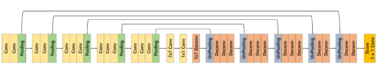
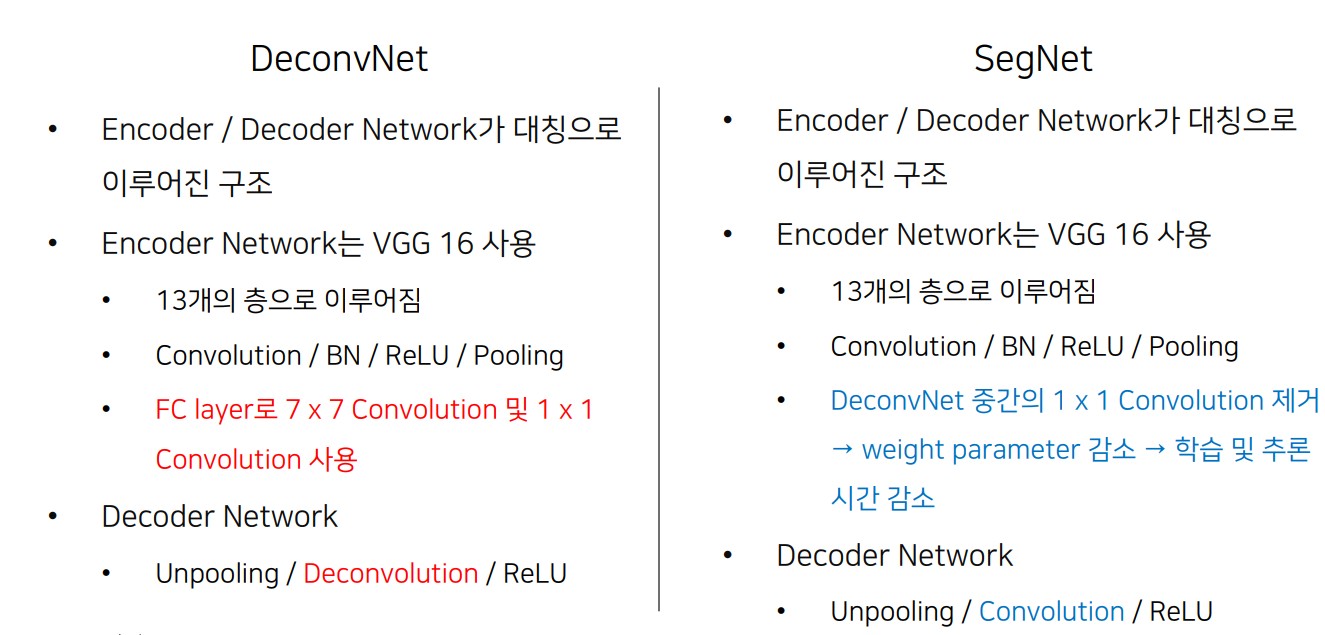
2.1 DeconvNet

Decoder를 Encoder와 대칭으로 만든 형태

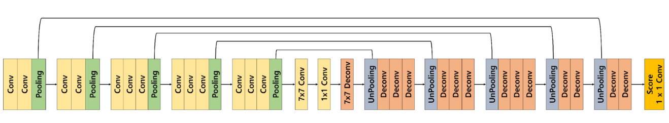
1. Convolution Network는 VGG16을 사용
• 13개의 층으로 이루어짐
• ReLU와 Pooling이 convolution 사이에서 이루어짐
• 7 x 7 Convolution 및 1 x 1 Convolution 을 활용
2. Deconvolution Network는 Unpooling, deconvolution, ReLU으로 이루어짐

Unpooling 이랑 Transposed convolution 이 반복.
• Unpooling은 디테일한 경계를 포착
• Transposed Convolution은 전반적인 모습을 포착

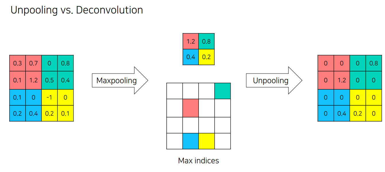
Unpooling

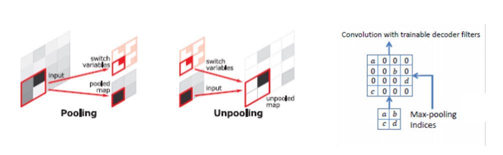
Pooling의 경우 노이즈를 제거하는 장점이 있지만, 그 과정에서 정보가 손실되는 문제가 생김
• Unpooling을 통해서 Pooling시에 지워진 경계에 정보를 기록했다가 복원
• 학습이 필요 없기 때문에 속도가 빠름
• 하지만 sparse한 activation map을 가지기 때문에 이를 채워 줄 필요가 있음

채우는 역할을 Transposed Convolution이 수행

한마디로 요약하면, 줄인걸 다시 채우는데 채우는 빈 공간은 Transposed convolution 이 할 것.

Deconvolution

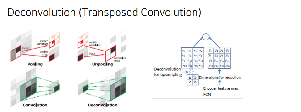
Deconvolution layers를 통해서 input object의 모양을 복원
• 순차적인 층의 구조가 다양한 수준의 모양을 잡아냄

얕은 층의 경우 전반적인 모습을 잡아냄
깊은 층의 경우 구체적인 모습을 잡아냄

Analysis of Deconvolution Network I

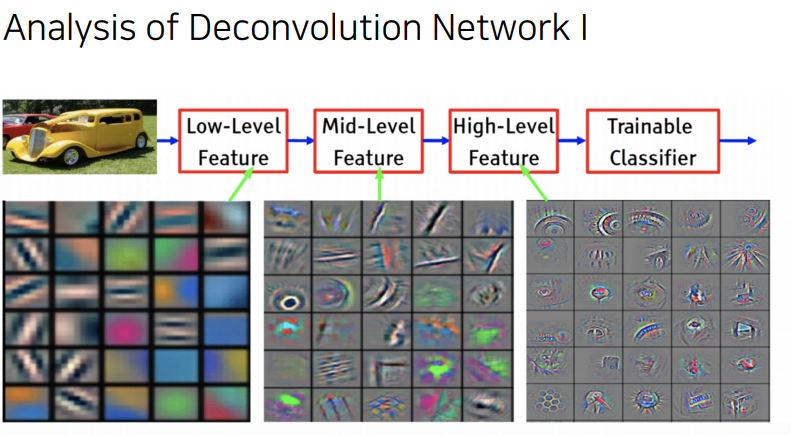
Low layer

직선 및 곡선, 색상 등의 낮은 수준의 특징
(local feature) 낮은층은 전반적인 특징(location , shape and region)

High layer

복잡하고 포괄적인 개체 정보가 활성화
(global feature) 깊은 층의 경우는 복잡한 패턴을 잡아냄.

Analysis of Deconvolution Network II

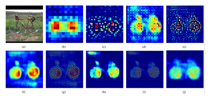
The image in (a) is an input, and the rest are the outputs from (b) the last 14 × 14 deconvolutional layer, (c) the 28 × 28 unpooling layer, (d) the last 28 × 28 deconvolutional layer, (e) the 56 × 56 unpooling layer, (f) the last 56 × 56 deconvolutional layer, (g) the 112 × 112 unpooling layer, (h) the last 112 × 112 deconvolutional layer, (i) the 224 × 224 unpooling layer and (j) the last 224 × 224 deconvolutional layer.

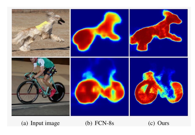
Deconvolution Network의 Activation map을 보면 층과 pooling 방법에 따라 다른 특징이 있음
• Unpooling의 경우 “example-specific”한 구조를 잡아냄 (자세한 구조를 잡아냄)
• Transposed Conv의 경우 “class-specific”한 구조를 잡아냄 (위의 구조에 빈 부분을 채워넣음)
• 실제로 둘을 병행시에 FCN보다 DeconvNet의 활성화 맵이 디테일해지는 모습을 볼 수 있음

Code

Convolution 부분

import torch.nn as nn

# CBR 함수 정의: Conv2d -> BatchNorm2d -> ReLU
def CBR(in_channels, out_channels, kernel_size=3, stride=1, padding=1):
    return nn.Sequential(
        nn.Conv2d(in_channels=in_channels, out_channels=out_channels, kernel_size=kernel_size, stride=stride, padding=padding),
        nn.BatchNorm2d(out_channels),
        nn.ReLU(inplace=True)
    )

# DCB 함수 정의: ConvTranspose2d -> BatchNorm2d -> ReLU
def DCB(in_channels, out_channels, kernel_size=3, stride=1, padding=1):
    return nn.Sequential(
        nn.ConvTranspose2d(in_channels=in_channels, out_channels=out_channels, kernel_size=kernel_size, stride=stride, padding=padding),
        nn.BatchNorm2d(out_channels),
        nn.ReLU(inplace=True)
    )

# 네트워크 정의
class Network(nn.Module):
    def __init__(self, num_classes):
        super(Network, self).__init__()

        # conv1
        self.conv1_1 = CBR(3, 64, 3, 1, 1)
        self.conv1_2 = CBR(64, 64, 3, 1, 1)
        self.pool1 = nn.MaxPool2d(kernel_size=2, stride=2, ceil_mode=True, return_indices=True)

        # conv2
        self.conv2_1 = CBR(64, 128, 3, 1, 1)
        self.conv2_2 = CBR(128, 128, 3, 1, 1)
        self.pool2 = nn.MaxPool2d(kernel_size=2, stride=2, ceil_mode=True, return_indices=True)

        # conv3
        self.conv3_1 = CBR(128, 256, 3, 1, 1)
        self.conv3_2 = CBR(256, 256, 3, 1, 1)
        self.conv3_3 = CBR(256, 256, 3, 1, 1)
        self.pool3 = nn.MaxPool2d(kernel_size=2, stride=2, ceil_mode=True, return_indices=True)

        # conv4
        self.conv4_1 = CBR(256, 512, 3, 1, 1)
        self.conv4_2 = CBR(512, 512, 3, 1, 1)
        self.conv4_3 = CBR(512, 512, 3, 1, 1)
        self.pool4 = nn.MaxPool2d(kernel_size=2, stride=2, ceil_mode=True, return_indices=True)

        # conv5
        self.conv5_1 = CBR(512, 512, 3, 1, 1)
        self.conv5_2 = CBR(512, 512, 3, 1, 1)
        self.conv5_3 = CBR(512, 512, 3, 1, 1)
        self.pool5 = nn.MaxPool2d(kernel_size=2, stride=2, ceil_mode=True, return_indices=True)

        # fc6
        self.fc6 = CBR(512, 4096, 7, 1, 0)
        self.drop6 = nn.Dropout2d(0.5)

        # fc7
        self.fc7 = CBR(4096, 4096, 1, 1, 0)
        self.drop7 = nn.Dropout2d(0.5)

        # score layer
        self.score_fr = nn.Conv2d(4096, num_classes, 1, 1, 0)

        # fc6 deconvolution for upsampling
        self.fc6_deconv = DCB(4096, 512, 7, 1, 0)

   def forward(self, x):
      # Encoding 단계
      h = self.conv1_1(x)
      h = self.conv1_2(h)
      h, pool1_indices = self.pool1(h)

      # 중략: conv2, conv3, conv4, conv5와 각 pool 레이어 수행
      # poolX_indices는 각 단계의 인덱스를 저장

      h = self.conv5_1(h)
      h = self.conv5_2(h)
      h = self.conv5_3(h)
      h, pool5_indices = self.pool5(h)

      # Decoding 단계
      h = self.unpool5(h, pool5_indices)
      h = self.deconv5_1(h)
      h = self.deconv5_2(h)
      h = self.deconv5_3(h)

      # 중략: unpool4 ~ unpool1까지 각 단계에서 디코딩 수행
      # 각 단계에서 deconvX_Y 레이어로 세부 정보를 추가

      h = self.unpool1(h, pool1_indices)
      h = self.deconv1_1(h)
      h = self.deconv1_2(h)

    # 최종 예측
    output = self.score_fr(h)
    return output

deconvolution 부분

import torch.nn as nn

# DCB (Deconvolution Block) 정의
def DCB(in_channels, out_channels, kernel_size=3, stride=1, padding=1):
    return nn.Sequential(
        nn.ConvTranspose2d(in_channels=in_channels, out_channels=out_channels, kernel_size=kernel_size, stride=stride, padding=padding),
        nn.BatchNorm2d(out_channels),
        nn.ReLU(inplace=True)
    )

class Network(nn.Module):
    def __init__(self, num_classes):
        super(Network, self).__init__()

        # Unpooling과 Deconvolution 레이어 정의
        # Unpool5과 Deconv5 블록
        self.unpool5 = nn.MaxUnpool2d(2, stride=2)
        self.deconv5_1 = DCB(512, 512, 3, 1, 1)
        self.deconv5_2 = DCB(512, 512, 3, 1, 1)
        self.deconv5_3 = DCB(512, 512, 3, 1, 1)

        # Unpool4과 Deconv4 블록
        self.unpool4 = nn.MaxUnpool2d(2, stride=2)
        self.deconv4_1 = DCB(512, 512, 3, 1, 1)
        self.deconv4_2 = DCB(512, 512, 3, 1, 1)
        self.deconv4_3 = DCB(512, 256, 3, 1, 1)

        # Unpool3과 Deconv3 블록
        self.unpool3 = nn.MaxUnpool2d(2, stride=2)
        self.deconv3_1 = DCB(256, 256, 3, 1, 1)
        self.deconv3_2 = DCB(256, 256, 3, 1, 1)
        self.deconv3_3 = DCB(256, 128, 3, 1, 1)

        # Unpool2과 Deconv2 블록
        self.unpool2 = nn.MaxUnpool2d(2, stride=2)
        self.deconv2_1 = DCB(128, 128, 3, 1, 1)
        self.deconv2_2 = DCB(128, 64, 3, 1, 1)

        # Unpool1과 Deconv1 블록
        self.unpool1 = nn.MaxUnpool2d(2, stride=2)
        self.deconv1_1 = DCB(64, 64, 3, 1, 1)
        self.deconv1_2 = DCB(64, 64, 3, 1, 1)

        # 최종 Score Layer
        self.score_fr = nn.Conv2d(64, num_classes, 1, 1, 0)

    def forward(self, x, indices):
        # 인덱스는 각 unpool 단계에서 사용
        x = self.unpool5(x, indices[4])
        x = self.deconv5_1(x)
        x = self.deconv5_2(x)
        x = self.deconv5_3(x)

        x = self.unpool4(x, indices[3])
        x = self.deconv4_1(x)
        x = self.deconv4_2(x)
        x = self.deconv4_3(x)

        x = self.unpool3(x, indices[2])
        x = self.deconv3_1(x)
        x = self.deconv3_2(x)
        x = self.deconv3_3(x)

        x = self.unpool2(x, indices[1])
        x = self.deconv2_1(x)
        x = self.deconv2_2(x)

        x = self.unpool1(x, indices[0])
        x = self.deconv1_1(x)
        x = self.deconv1_2(x)

        x = self.score_fr(x)
        return x

2.2 SegNet

SegNet 동기

Road Scene Understanding applications라는 분야에서 Semantic Segmentation을 수행하기 위해 모델이 필요한 능력에 대한 고민
• 특히, 자율 주행에 있어 차량, 도로, 차선, 건물, 보도, 하늘, 사람 등의 class를 빠르고, 정확하게 구분할 수 있어야함
-> 속도를 빠르게 하는것에 초첨!

DeconvNet과 다른점

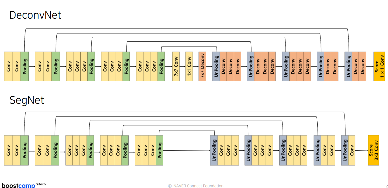
파라미터 줄이고, Unpolling 학습 x, sparse -> dense, 마지막 deconv 없애고 score를 3x3 conv 함

특징	SegNet	DeconvNet
파라미터 수	적음	많음
Unpooling 방식	Pooling 인덱스를 이용한 비학습형 Unpooling	학습형 Deconvolution
Sparse to Dense	Sparse 인덱스를 Dense한 피처 맵으로 변환	ConvTranspose로 Dense 변환
마지막 레이어	3x3 Convolution (Score Layer)	Deconvolution (ConvTranspose)

Code

import torch.nn as nn

# CBR 함수 정의 (Convolution + BatchNorm + ReLU)
def CBR(in_channels, out_channels, kernel_size=3, stride=1, padding=1):
    return nn.Sequential(
        nn.Conv2d(in_channels=in_channels, out_channels=out_channels, kernel_size=kernel_size, stride=stride, padding=padding),
        nn.BatchNorm2d(num_features=out_channels),
        nn.ReLU()
    )

class SegNet(nn.Module):
    def __init__(self, num_classes):
        super(SegNet, self).__init__()
        
        # Encoder
        # conv1
        self.cbr1_1 = CBR(3, 64, 3, 1, 1)
        self.cbr1_2 = CBR(64, 64, 3, 1, 1)
        self.pool1 = nn.MaxPool2d(2, stride=2, ceil_mode=True, return_indices=True)

        # conv2
        self.cbr2_1 = CBR(64, 128, 3, 1, 1)
        self.cbr2_2 = CBR(128, 128, 3, 1, 1)
        self.pool2 = nn.MaxPool2d(2, stride=2, ceil_mode=True, return_indices=True)

        # conv3
        self.cbr3_1 = CBR(128, 256, 3, 1, 1)
        self.cbr3_2 = CBR(256, 256, 3, 1, 1)
        self.cbr3_3 = CBR(256, 256, 3, 1, 1)
        self.pool3 = nn.MaxPool2d(2, stride=2, ceil_mode=True, return_indices=True)

        # conv4
        self.cbr4_1 = CBR(256, 512, 3, 1, 1)
        self.cbr4_2 = CBR(512, 512, 3, 1, 1)
        self.cbr4_3 = CBR(512, 512, 3, 1, 1)
        self.pool4 = nn.MaxPool2d(2, stride=2, ceil_mode=True, return_indices=True)

        # conv5
        self.cbr5_1 = CBR(512, 512, 3, 1, 1)
        self.cbr5_2 = CBR(512, 512, 3, 1, 1)
        self.cbr5_3 = CBR(512, 512, 3, 1, 1)
        self.pool5 = nn.MaxPool2d(2, stride=2, ceil_mode=True, return_indices=True)

        # Decoder
        # deconv5
        self.unpool5 = nn.MaxUnpool2d(2, stride=2)
        self.dcbr5_3 = CBR(512, 512, 3, 1, 1)
        self.dcbr5_2 = CBR(512, 512, 3, 1, 1)
        self.dcbr5_1 = CBR(512, 512, 3, 1, 1)

        # deconv4
        self.unpool4 = nn.MaxUnpool2d(2, stride=2)
        self.dcbr4_3 = CBR(512, 512, 3, 1, 1)
        self.dcbr4_2 = CBR(512, 512, 3, 1, 1)
        self.dcbr4_1 = CBR(512, 256, 3, 1, 1)

        # deconv3
        self.unpool3 = nn.MaxUnpool2d(2, stride=2)
        self.dcbr3_3 = CBR(256, 256, 3, 1, 1)
        self.dcbr3_2 = CBR(256, 256, 3, 1, 1)
        self.dcbr3_1 = CBR(256, 128, 3, 1, 1)

        # deconv2
        self.unpool2 = nn.MaxUnpool2d(2, stride=2)
        self.dcbr2_2 = CBR(128, 128, 3, 1, 1)
        self.dcbr2_1 = CBR(128, 64, 3, 1, 1)

        # deconv1
        self.unpool1 = nn.MaxUnpool2d(2, stride=2)
        self.deconv1_1 = CBR(64, 64, 3, 1, 1)

        # Score layer
        self.score_fr = nn.Conv2d(64, num_classes, 3, 1, 1)

    def forward(self, x):
        # Encoder
        h = self.cbr1_1(x)
        h = self.cbr1_2(h)
        h, pool1_indices = self.pool1(h)

        h = self.cbr2_1(h)
        h = self.cbr2_2(h)
        h, pool2_indices = self.pool2(h)

        h = self.cbr3_1(h)
        h = self.cbr3_2(h)
        h = self.cbr3_3(h)
        h, pool3_indices = self.pool3(h)

        h = self.cbr4_1(h)
        h = self.cbr4_2(h)
        h = self.cbr4_3(h)
        h, pool4_indices = self.pool4(h)

        h = self.cbr5_1(h)
        h = self.cbr5_2(h)
        h = self.cbr5_3(h)
        h, pool5_indices = self.pool5(h)

        # Decoder
        h = self.unpool5(h, pool5_indices)
        h = self.dcbr5_3(h)
        h = self.dcbr5_2(h)
        h = self.dcbr5_1(h)

        h = self.unpool4(h, pool4_indices)
        h = self.dcbr4_3(h)
        h = self.dcbr4_2(h)
        h = self.dcbr4_1(h)

        h = self.unpool3(h, pool3_indices)
        h = self.dcbr3_3(h)
        h = self.dcbr3_2(h)
        h = self.dcbr3_1(h)

        h = self.unpool2(h, pool2_indices)
        h = self.dcbr2_2(h)
        h = self.dcbr2_1(h)

        h = self.unpool1(h, pool1_indices)
        h = self.deconv1_1(h)

        output = self.score_fr(h)
        return output

2.3 DeconvNet vs SegNet

3. Skip Connection을 적용한 models

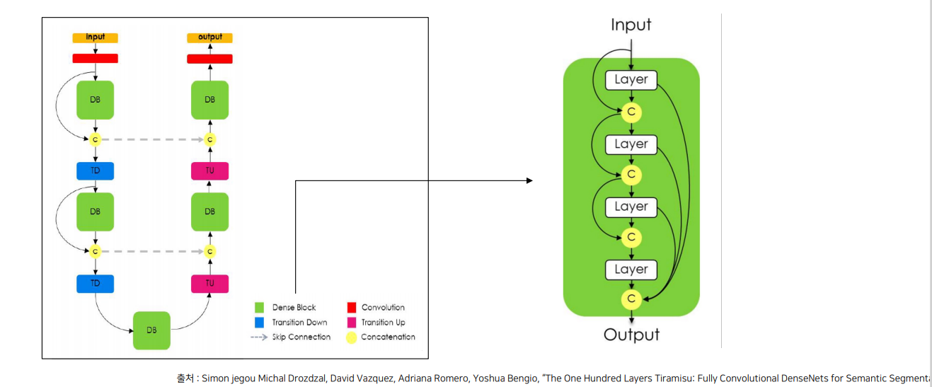
3.1 FC DenseNet

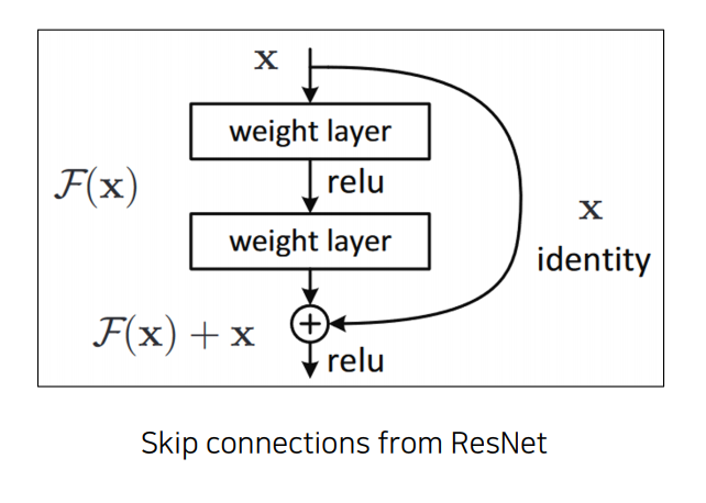
Skip Connection

Neural network에서 이전 layer의 output을 일부 layer를 건너 뛴 후의 layer에게 입력으로 제공하는 것

Dense Skip Connection

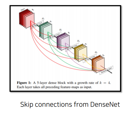
DenseNet의 스킵 연결은 모든 이전 레이어의 출력을 다음 레이어에 전달하는 밀집 연결 방식을 사용하여, 네트워크의 정보 흐름을 극대화하고, 학습 효율성을 높임

Architecture

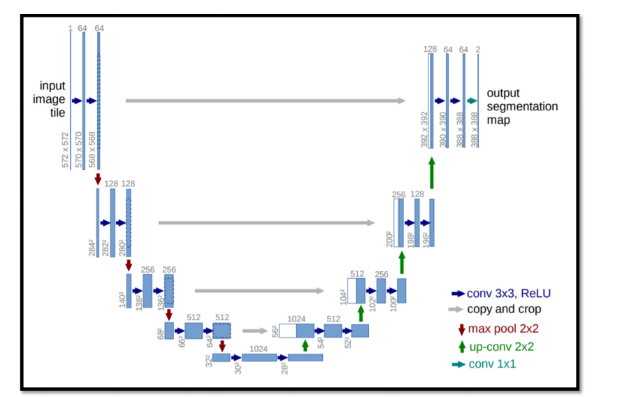
3.2 Unet

매우 중요함. 6강에서 다시봄.
여기서는
encoder에서 decoder로 정보를 주는 부분이 4개가 있다 정도만 학습.

4. Receptive Field를 확장시킨 models

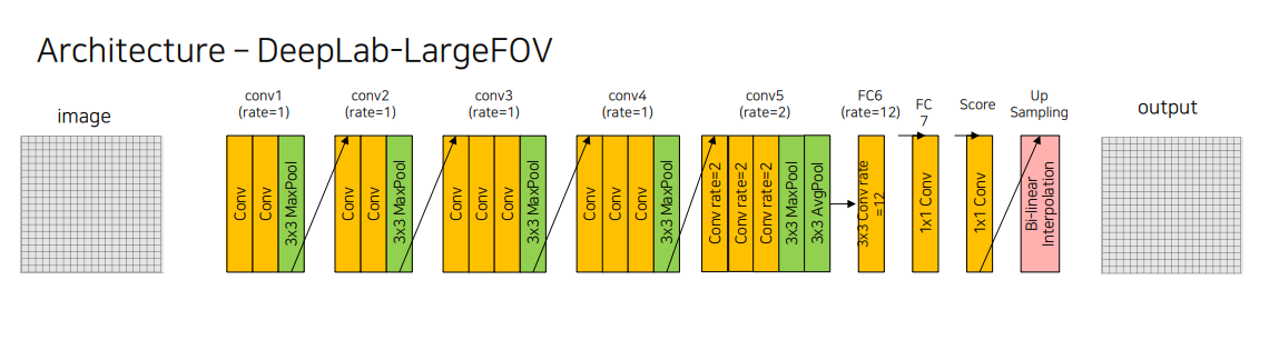
4.1 DeepLab v1

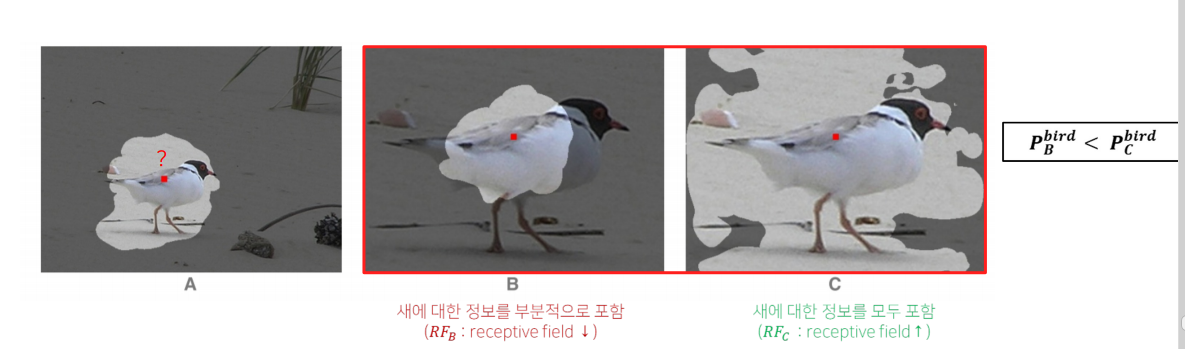
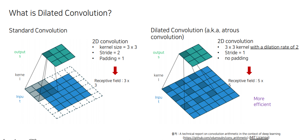
Why the receptive field is so important?

receptive field란 뉴런이 얼마만큼의 영역을 바라보고 있는 등에 대한 정보영역.

case1 : B와 C중에 누가 더 새라고 예측할까? ->C

receptive field 를 통해 C에서 새에 대한 정보를 더 많이 받았으므로.

case2 : 아래 image에서 receptive filde가 작은 segmentation 을 진행한다면?

receptive field 가 bus 에 대한 정보를 다 포함하지 못하므로 예측 정확도가 낮음

conv -> MaxPooling -> Conv반복하면, 효율적으로 Receptive field를 넓힐 수 있음.

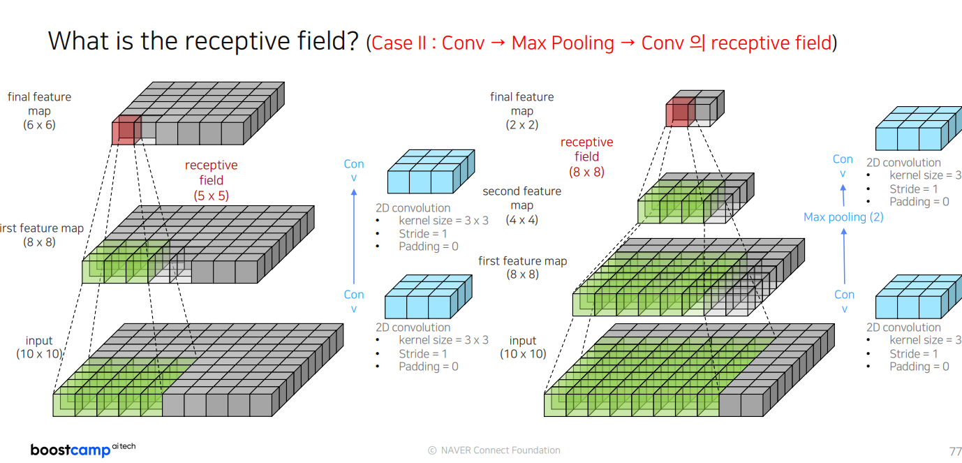
그러나 Resolution 측면에서는, low feature resolution 을 가지는 문제점이 있음

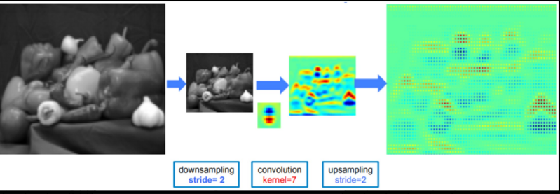
이미지의 크기를 줄이지 않고 파라미터수도 변함이 없는 채로 Receptive field만 넓게 하는 방식은 없을까?

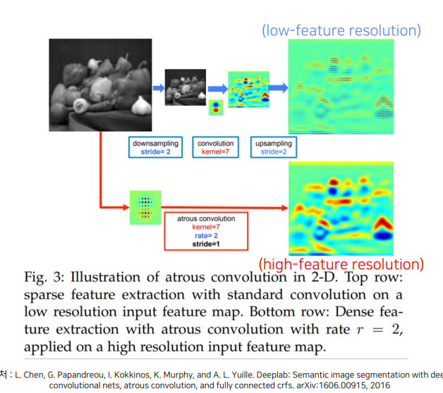
downsampling, upsampling 없앰. 이후 high -feature resolution

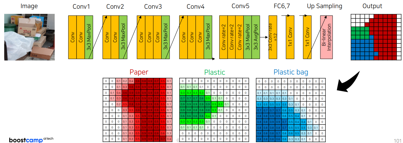
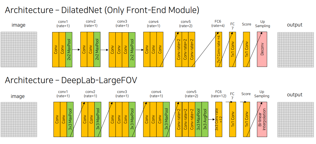
Architecture

import torch
import torch.nn as nn
import torch.nn.functional as F

# Convolution + ReLU Block
def conv_relu(in_ch, out_ch, size=3, rate=1):
    conv_relu = nn.Sequential(
        nn.Conv2d(in_channels=in_ch, out_channels=out_ch, kernel_size=size, stride=1, padding=rate, dilation=rate),
        nn.ReLU()
    )
    return conv_relu

# VGG16 Backbone Definition
class VGG16(nn.Module):
    def __init__(self):
        super(VGG16, self).__init__()
        self.features1 = nn.Sequential(
            conv_relu(3, 64, 3, 1),
            conv_relu(64, 64, 3, 1),
            nn.MaxPool2d(3, stride=2, padding=1)
        )
        self.features2 = nn.Sequential(
            conv_relu(64, 128, 3, 1),
            conv_relu(128, 128, 3, 1),
            nn.MaxPool2d(3, stride=2, padding=1)
        )
        self.features3 = nn.Sequential(
            conv_relu(128, 256, 3, 1),
            conv_relu(256, 256, 3, 1),
            conv_relu(256, 256, 3, 1),
            nn.MaxPool2d(3, stride=2, padding=1)
        )
        self.features4 = nn.Sequential(
            conv_relu(256, 512, 3, 1),
            conv_relu(512, 512, 3, 1),
            conv_relu(512, 512, 3, 1),
            nn.MaxPool2d(3, stride=2, padding=1)
        )
        self.features5 = nn.Sequential(
            conv_relu(512, 512, 3, rate=2),
            conv_relu(512, 512, 3, rate=2),
            conv_relu(512, 512, 3, rate=2),
            nn.MaxPool2d(3, stride=1, padding=1),
            nn.AvgPool2d(3, stride=1, padding=1)
        )

# Classifier Definition
class Classifier(nn.Module):
    def __init__(self, num_classes):
        super(Classifier, self).__init__()
        self.classifier = nn.Sequential(
            conv_relu(512, 1024, 3, rate=12),
            nn.Dropout2d(0.5),
            conv_relu(1024, 1024, 1, 1),
            nn.Dropout2d(0.5),
            nn.Conv2d(1024, num_classes, 1)
        )

    def forward(self, x):
        out = self.classifier(x)
        return out

# DeepLabV1 Definition
class DeepLabV1(nn.Module):
    def __init__(self, backbone, classifier, upsampling=8):
        super(DeepLabV1, self).__init__()
        self.backbone = backbone
        self.classifier = classifier
        self.upsampling = upsampling

    def forward(self, x):
        x = self.backbone(x)
        _, _, feature_map_h, feature_map_w = x.size()
        x = self.classifier(x)
        x = F.interpolate(x, size=(feature_map_h * self.upsampling, feature_map_w * self.upsampling), mode="bilinear", align_corners=True)
        return x

# Example of model instantiation
backbone = VGG16()
classifier = Classifier(num_classes=21)
model = DeepLabV1(backbone, classifier)

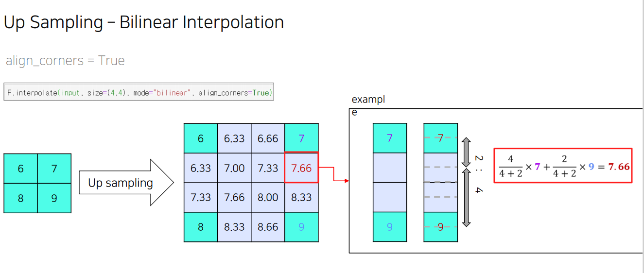
bilinearInteporation 이란?

새로운 이미지의 픽셀 값을 원본 이미지에서 가장 가까운 네 개의 픽셀 값을 기반으로 가중 평균하여 계산하는 방식

Dense Conditional Random Field (Dense CRF, a.k.a Fully-Connected CRF)

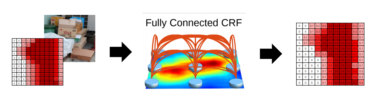
Bilinear Interpolation 으로는 픽셀 단위의 정교한 segmentation이 불가능
이를 개선하기 위한 후처리 방법 � Dense CRF

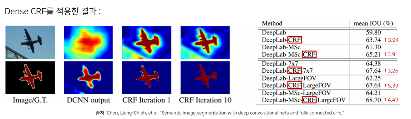
Dense Conditional Random Field (Dense CRF, a.k.a Fully-Connected CRF) 과정

Step 1) DeepLab v1을 이용해 segmentation 수행

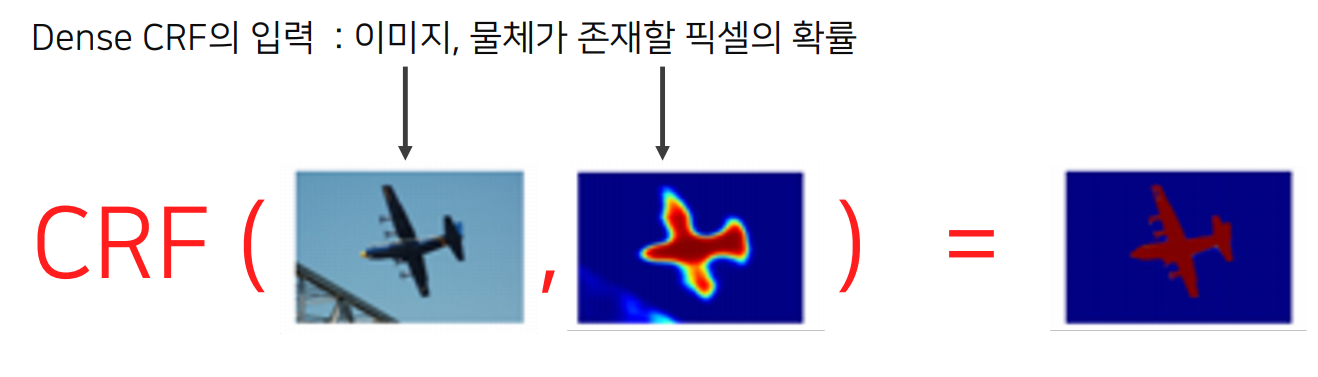
Step 2) 계산된 확률 및 이미지를 CRF에 입력

색상이 유사한 픽셀이 가까이 위치하면 같은 범주에 속함
색상이 유사해도 픽셀의 거리가 멀다면 같은 범주에 속하지 않음

Step 3) 여러 번 반복 수행

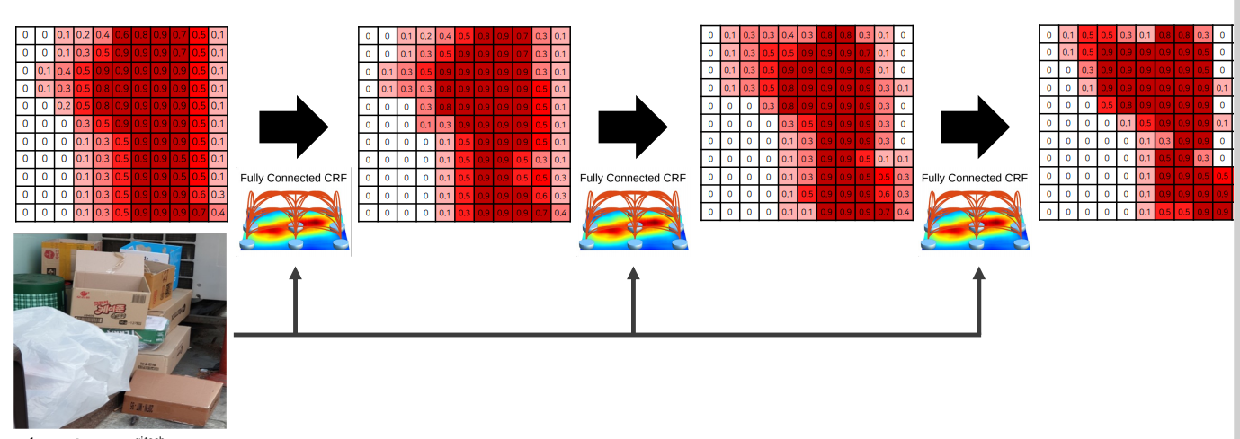
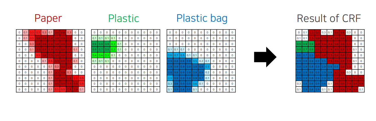
Step 4) 다른 카테고리에 대해 같은 과정 수행

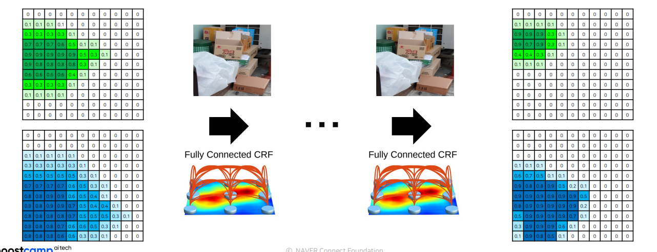
Step 5) 각 픽셀 별 가장 높은 확률을 갖는 카테고리 선택하여 최종 결과 도출

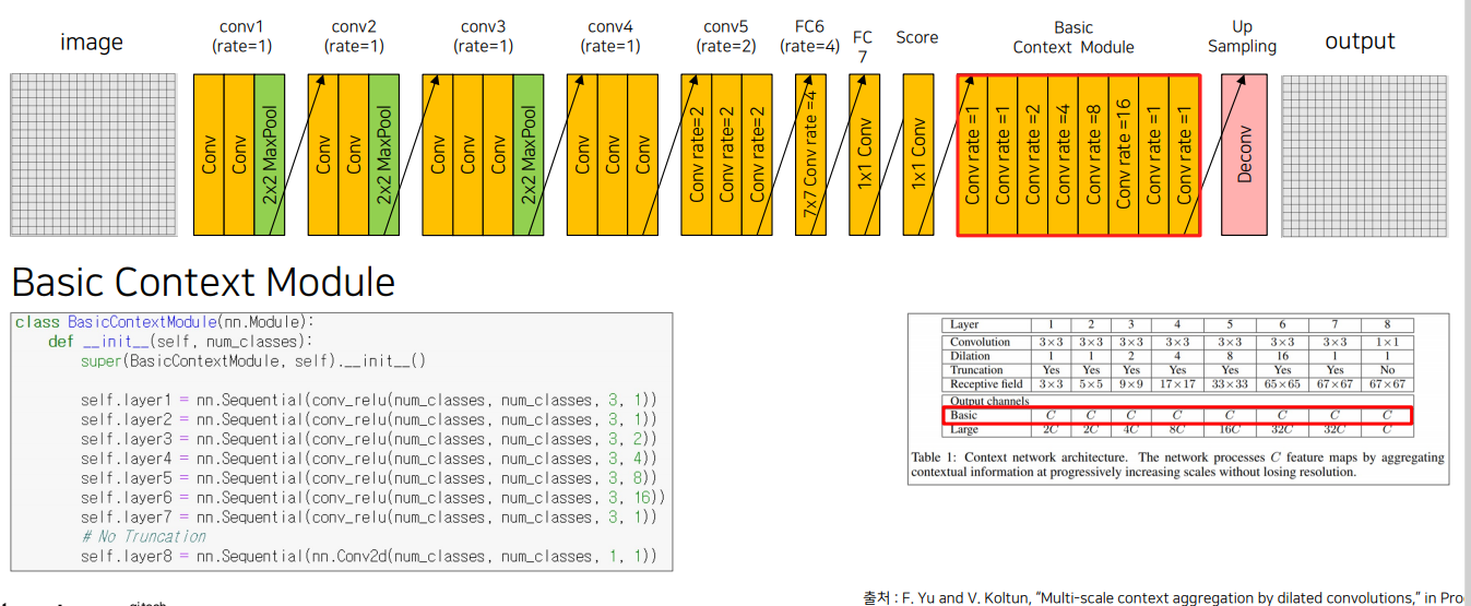
4.2 DilatedNet

def conv_relu(in_ch, out_ch, size=3, rate=1):
    conv_relu = nn.Sequential(
        nn.Conv2d(in_channels=in_ch,
                  out_channels=out_ch,
                  kernel_size=size,
                  stride=1,
                  padding=rate,
                  dilation=rate),
        nn.ReLU()
    )
    return conv_relu

class VGG16(nn.Module):
    def __init__(self):
        super(VGG16, self).__init__()
        self.features1 = nn.Sequential(
            conv_relu(3, 64, 3, 1),
            conv_relu(64, 64, 3, 1),
            nn.MaxPool2d(2, stride=2, padding=0)  # 1/2
        )
        self.features3 = nn.Sequential(
            conv_relu(128, 256, 3, 1),
            conv_relu(256, 256, 3, 1),
            conv_relu(256, 256, 3, 1),
            nn.MaxPool2d(2, stride=2, padding=0)  # 1/8
        )
        self.features4 = nn.Sequential(
            conv_relu(256, 512, 3, 1),
            conv_relu(512, 512, 3, 1),
            conv_relu(512, 512, 3, 1)
        )
        self.features5 = nn.Sequential(
            conv_relu(512, 512, 3, 2),
            conv_relu(512, 512, 3, 2),
            conv_relu(512, 512, 3, 2)
        )
class classifier(nn.Module):
    def __init__(self, num_classes):
        super(classifier, self).__init__()
        self.classifier = nn.Sequential(
            nn.Conv2d(512, 4096, kernel_size=7, dilation=4, padding=12),
            nn.ReLU(),
            nn.Dropout2d(0.5),
            nn.Conv2d(4096, 4096, kernel_size=1),
            nn.ReLU(),
            nn.Dropout2d(0.5),
            nn.Conv2d(4096, num_classes, kernel_size=1)
        )

    def forward(self, x):
        out = self.classifier(x)
        return out
class DilatedNetFront(nn.Module):
    def __init__(self, backbone, classifier, context_module):
        super(DilatedNetFront, self).__init__()
        self.backbone = backbone
        self.classifier = classifier
        self.context_module = context_module
        self.deconv = nn.ConvTranspose2d(in_channels=11, out_channels=11,
                                         kernel_size=16, stride=8, padding=4)

    def forward(self, x):
        x = self.backbone(x)
        x = self.classifier(x)
        out = self.deconv(x)
        return out

정리

FCN은 Object의 디테일한 모습에 대해 예측을 잘 못하며, DeconvNet은 Encoder-Decoder 구조를 통해서 FCN의 한계를 극복하려고 했습니다. Dilated Convolution은 Receptive Field를 넓혀주는 효과가 있습니다.
DeconvNet에서는 Convolution Network는 VGG16을 사용합니다.
주로 Receptive field가 object에 대한 정보를 다 포함하지 못하므로 예측 정확도가 낮을 수 있다고 알려져 있다.