Stanley Method

1. Stanley Method란?

• 2005년 Darpa Grand Challenge에서 우승을 차지한 Standford University 팀이 사용한 사용한 Contoller

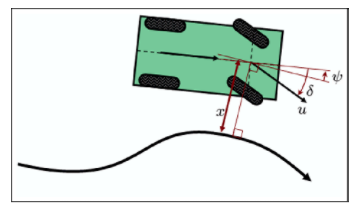
• Pure pursuit과는 다르게 앞바퀴를 reference point로 잡음

• Cross track Error와 heading error 를 고려하여 제어를 한다.

2. Formulation

• $\psi(t)$ 는 heading error를 잡아주고, $\arctan(\frac{kx(t)}{u(t)})$ 는 CTR 를 잡아주는 역할

• 속도가 낮을 경우를 보정하기 위해 다음과 같이 $k_s$를 추가할 수도 있음.

  $\delta(t) = \psi(t) + \arctan(\frac{kx(t)}{k_s +u(t)})$

3. 예시

• heading error가 클시

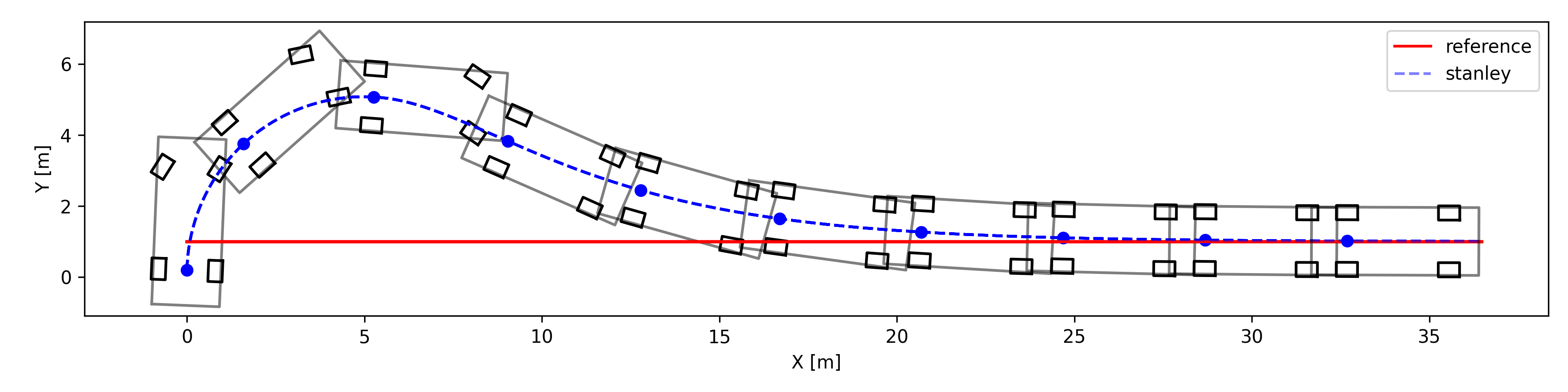
• CTR이 클시

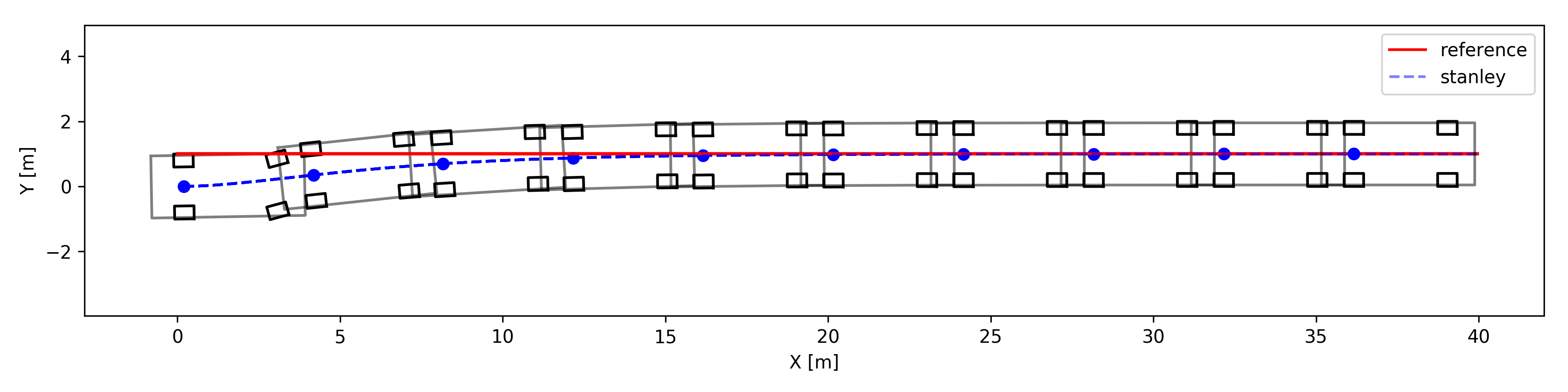
4. 파이썬 구현

import numpy as np
import matplotlib.pyplot as plt

# paramters
dt = 0.1

k = 0.5  # control gain

# GV70 PARAMETERS
LENGTH = 4.715
WIDTH = 1.910
L = 2.875
BACKTOWHEEL = 1.0
WHEEL_LEN = 0.3  # [m]
WHEEL_WIDTH = 0.2  # [m]
TREAD = 0.8  # [m]

class VehicleModel(object):
    def __init__(self, x=0.0, y=0.0, yaw=0.0, v=0.0):
        self.x = x
        self.y = y
        self.yaw = yaw
        self.v = v

        self.max_steering = np.radians(30)

    def update(self, steer, a=0):
        steer = np.clip(steer, -self.max_steering, self.max_steering)
        self.x += self.v * np.cos(self.yaw) * dt
        self.y += self.v * np.sin(self.yaw) * dt
        self.yaw += self.v / L * np.tan(steer) * dt
        self.yaw = self.yaw % (2.0 * np.pi)
        self.v += a * dt


def normalize_angle(angle):
    while angle > np.pi:
        angle -= 2.0 * np.pi

    while angle < -np.pi:
        angle += 2.0 * np.pi

    return angle


def stanley_control(x, y, yaw, v, map_xs, map_ys, map_yaws):
    # find nearest point
    min_dist = 1e9
    min_index = 0
    n_points = len(map_xs)

    front_x = x + L * np.cos(yaw)
    front_y = y + L * np.sin(yaw)

    for i in range(n_points):
        dx = front_x - map_xs[i]
        dy = front_y - map_ys[i]

        dist = np.sqrt(dx * dx + dy * dy)
        if dist < min_dist:
            min_dist = dist
            min_index = i

    # compute cte at front axle
    map_x = map_xs[min_index]
    map_y = map_ys[min_index]
    map_yaw = map_yaws[min_index]
    dx = map_x - front_x
    dy = map_y - front_y

    perp_vec = [np.cos(yaw + np.pi/2), np.sin(yaw + np.pi/2)]
    cte = np.dot([dx, dy], perp_vec)

    # control law
    yaw_term = normalize_angle(map_yaw - yaw)
    cte_term = np.arctan2(k*cte, v)

    # steering
    steer = yaw_term + cte_term
    return steer


# map
target_y = 1.0
map_xs = np.linspace(0, 500, 500)
map_ys = np.ones_like(map_xs) * target_y
map_yaws = np.ones_like(map_xs) * 0.0

# vehicle
model = VehicleModel(x=0.0, y=0.0, yaw=0.0, v=2.0)
steer = 0


xs = []
ys = []
yaws = []
steers = []
ts = []
for step in range(200):
    # plt.clf()
    t = step * dt

    steer = stanley_control(model.x, model.y, model.yaw, model.v, map_xs, map_ys, map_yaws)
    steer = np.clip(steer, -model.max_steering, model.max_steering)
    model.update(steer)

    xs.append(model.x)
    ys.append(model.y)
    yaws.append(model.yaw)
    ts.append(t)
    steers.append(steer)

# plot car
plt.figure(figsize=(12, 3))
plt.plot([0, xs[-1]], [target_y, target_y], 'r-', label="reference")
plt.plot(xs, ys, 'b--', alpha=0.5, label="stanley")
for i in range(len(xs)):
    # plt.clf()
    if i % 20 == 0:
        plt.plot([0, xs[-1]], [target_y, target_y], 'r-')
        plt.plot(xs, ys, 'b--', alpha=0.5)
        x = xs[i]
        y = ys[i]
        yaw = yaws[i]
        steer = steers[i]

        outline = np.array([[-BACKTOWHEEL, (LENGTH - BACKTOWHEEL), (LENGTH - BACKTOWHEEL), -BACKTOWHEEL, -BACKTOWHEEL],
                            [WIDTH / 2, WIDTH / 2, - WIDTH / 2, -WIDTH / 2, WIDTH / 2]])
        fr_wheel = np.array([[WHEEL_LEN, -WHEEL_LEN, -WHEEL_LEN, WHEEL_LEN, WHEEL_LEN],
                             [-WHEEL_WIDTH, -WHEEL_WIDTH, WHEEL_WIDTH, WHEEL_WIDTH, -WHEEL_WIDTH]])

        rr_wheel = np.copy(fr_wheel)
        fl_wheel = np.copy(fr_wheel)
        rl_wheel = np.copy(rr_wheel)

        Rot1 = np.array([[np.cos(yaw), np.sin(yaw)],
                         [-np.sin(yaw), np.cos(yaw)]])
        Rot2 = np.array([[np.cos(steer+yaw), np.sin(steer+yaw)],
                         [-np.sin(steer+yaw), np.cos(steer+yaw)]])

        fr_wheel = (fr_wheel.T.dot(Rot2)).T
        fl_wheel = (fl_wheel.T.dot(Rot2)).T
        fr_wheel[0, :] += L * np.cos(yaw) - TREAD * np.sin(yaw)
        fl_wheel[0, :] += L * np.cos(yaw) + TREAD * np.sin(yaw)
        fr_wheel[1, :] += L * np.sin(yaw) + TREAD * np.cos(yaw)
        fl_wheel[1, :] += L * np.sin(yaw) - TREAD * np.cos(yaw)
        rr_wheel[1, :] += TREAD
        rl_wheel[1, :] -= TREAD

        outline = (outline.T.dot(Rot1)).T
        rr_wheel = (rr_wheel.T.dot(Rot1)).T
        rl_wheel = (rl_wheel.T.dot(Rot1)).T

        outline[0, :] += x
        outline[1, :] += y
        fr_wheel[0, :] += x
        fr_wheel[1, :] += y
        rr_wheel[0, :] += x
        rr_wheel[1, :] += y
        fl_wheel[0, :] += x
        fl_wheel[1, :] += y
        rl_wheel[0, :] += x
        rl_wheel[1, :] += y

        plt.plot(np.array(outline[0, :]).flatten(),
                 np.array(outline[1, :]).flatten(), 'k-', alpha=0.5)
        plt.plot(np.array(fr_wheel[0, :]).flatten(),
                 np.array(fr_wheel[1, :]).flatten(), 'k-')
        plt.plot(np.array(rr_wheel[0, :]).flatten(),
                 np.array(rr_wheel[1, :]).flatten(), 'k-')
        plt.plot(np.array(fl_wheel[0, :]).flatten(),
                 np.array(fl_wheel[1, :]).flatten(), 'k-')
        plt.plot(np.array(rl_wheel[0, :]).flatten(),
                 np.array(rl_wheel[1, :]).flatten(), 'k-')
        plt.plot(x, y, "bo")
        plt.axis("equal")
        # plt.pause(0.1)
plt.xlabel("X [m]")
plt.ylabel("Y [m]")
plt.legend(loc="best")
plt.tight_layout()
plt.savefig("stanley_method.png", dpi=300)
plt.show()

---

• https://www.researchgate.net/publication/220648006_Stanley_The_robot_that_won_the_DARPA_Grand_Challenge