# 전처리
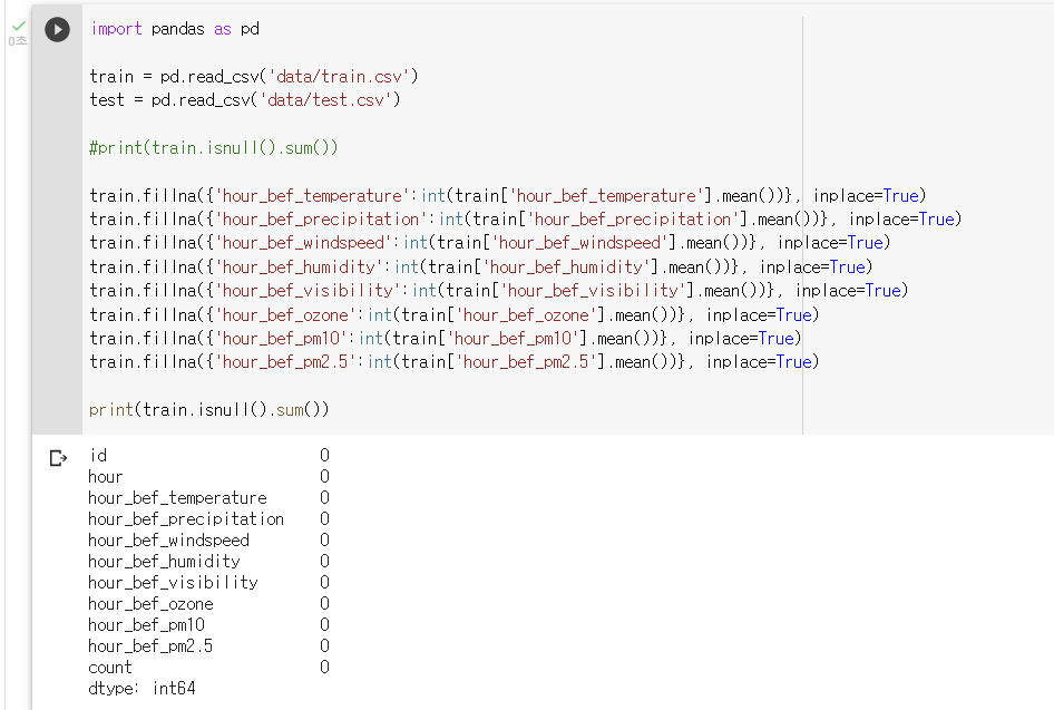
1. 결측치 평균으로 대체 (fillna({mean}))
: 각 피쳐의 평균값으로 결측치 대체
: df.fillna({'칼럼명':int(df['칼럼명'].mean)}, inplace=True)
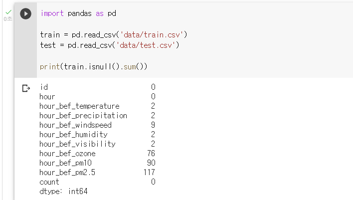
: 결측치가 있는 피쳐 살펴보기
print(train.isnull().sum())
: 결측치 평균값으로 대체하기train.fillna({'hour_bef_temperature':int(train['hour_bef_temperature'].mean())}, inplace=True) train.fillna({'hour_bef_precipitation':int(train['hour_bef_precipitation'].mean())}, inplace=True) train.fillna({'hour_bef_windspeed':int(train['hour_bef_windspeed'].mean())}, inplace=True) train.fillna({'hour_bef_humidity':int(train['hour_bef_humidity'].mean())}, inplace=True) train.fillna({'hour_bef_visibility':int(train['hour_bef_visibility'].mean())}, inplace=True) train.fillna({'hour_bef_ozone':int(train['hour_bef_ozone'].mean())}, inplace=True) train.fillna({'hour_bef_pm10':int(train['hour_bef_pm10'].mean())}, inplace=True) train.fillna({'hour_bef_pm2.5':int(train['hour_bef_pm2.5'].mean())}, inplace=True)
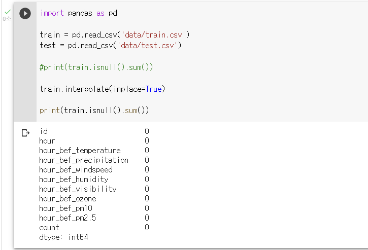
2. 결측치 보간법으로 대체 (interpolate())
: 피쳐의 정보성을 강조하기 위해 보간법을 사용해 결측치 대체
: Lv2 에서 다루고 있는 따릉이 데이터의 경우 피쳐들은 기상정보들이며 데이터의 순서는 시간 순서이다.
: 따라서 결측치들을 이전 행(직전시간)과 다음 행(직후시간)의 평균으로 보간하는 것은 상당히 합리적이다.
: Python pandas 의 interpolate() method 를 사용해 구현
: df.interpolate(inplace=True)
: 결측치 보간법으로 대체하기
train.interpolate(inplace=True)
# 모델링
1. 랜덤포레스트 개념, 선언 (RandomForestRegressor())
: 랜덤포레스트는 여러 개의 의사결정나무를 만들어서 이들의 평균으로 예측의 성능을 높이는 방법이다.
: 앙상블(Ensemble) 기법이라고도 한다.
: 주어진 하나의 데이터로부터 여러 개의 랜덤 데이터셋을 추출해, 각 데이터셋을 통해 모델을 여러 개 만들 수 있다.
: from sklearn.ensemble import RandomForestRegressor
model = RandomForestRegressor()
: sklearn.ensemble 로부터 RandomForestRegressor 를 불러와 모델을 선언하는 코드 작성하기
from sklearn.ensemble import RandomForestRegressor
model = RandomForestRegressor()
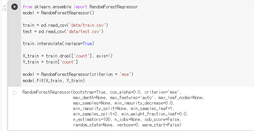
2. 랜덤포레스트를 평가척도에 맞게 학습 (criterion='mse')
: 랜덤포레스트 모듈의 옵션 중 criterion 옵션을 통해 어떤 평가척도를 기준으로 훈련할 것인지 정할 수 있다.
: 따릉이 대회의 평가지표는 RMSE이다.
: RMSE 는 MSE 평가지표에 루트를 씌운 것으로서, 모델을 선언할 때 criterion = ‘mse’ 옵션으로 구현할 수 있다.
: model = RandomForestRegressor(criterion = 'mse')

: count 피쳐를 제외한 X_train df 와 count 피쳐만을 가진 Y_train df 를 생성하는 코드 작성하기
X_train = train.drop(['count'], axis=1)
Y_train = train['count']
: 파이썬 랜덤포레스트를 따릉이 대회의 평가지표(=RMSE)에 맞게 학습하는 모델을 선언하고 모델을 훈련시키는 코드 작성
model = RandomForestRegressor(criterion = 'mse')
model.fit(X_train, Y_train)
# 튜닝
1. 랜덤포레스트 변수중요도 확인 (featureimportances)
: fit() 으로 모델이 학습되고 나면 featureimportances 속성(attribute) 으로 변수의 중요도를 파악할 수 있다.
: 변수의 중요도란 예측변수를 결정할 때 각 피쳐가 얼마나 중요한 역할을 하는지에 대한 척도이다.
: 변수의 중요도가 낮다면 해당 피쳐를 제거하는 것이 모델의 성능을 높일 수 있다.
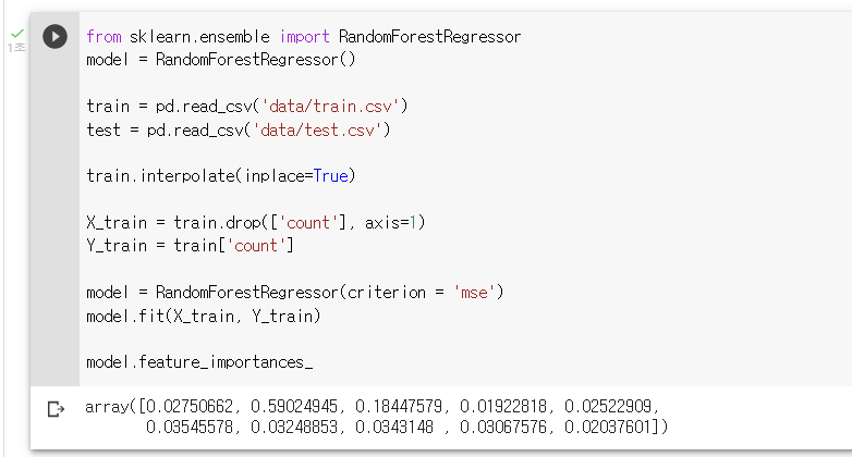
: model.feature_importances__
: 랜덤포레스트모델 예측변수의 중요도를 출력하는 코드 작성하기
model.feature_importances_
2. 변수 제거 (drop())
: 변수중요도가 낮은 피쳐를 파악하고 나면 차례대로 하나씩 피쳐를 제거하면서 모델을 새로 훈련할 수 있다.
: id 피쳐는 예측에 의미가 없는 피쳐이다.
: id 와 count 를 drop 한 X_train_1 훈련 df 을 새로 생성한다.
: 예측을 할 때 test 는 훈련 셋과 동일한 피쳐를 가져야 한다. 따라서 동일하게 피쳐를 drop 한 test_1 df 를 생성해준다.
: hour_bef_windspeed 와 hour_bef_pm2.5 피쳐에 관하여도 추가로 drop 을 수행하면서 위의 과정을 반복해보면 총 3 쌍의 X_train 셋과 test 셋이 생성된다.
: 각 모델로 예측한 예측값들을 submission 에 저장한 후, 리더보드에 제출해 점수를 비교해볼것 !
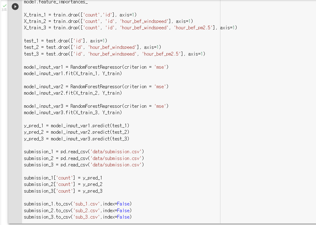
: X_train 에서 drop 할 피쳐의 경우에 수 대로 3개의 X_train 을 생성하기
X_train_1 = train.drop(['count','id'], axis=1)
X_train_2 = train.drop(['count', 'id', 'hour_bef_windspeed'], axis=1)
X_train_3 = train.drop(['count', 'id', 'hour_bef_windspeed', 'hour_bef_pm2.5'], axis=1)
: 각 train 에 따라 동일하게 피쳐를 drop 한 test 셋들을 생성하기
test_1 = test.drop(['id'], axis=1)
test_2 = test.drop(['id', 'hour_bef_windspeed'], axis=1)
test_3 = test.drop(['id', 'hour_bef_windspeed', 'hour_bef_pm2.5'], axis=1)
: 각 X_train에 대해 모델 훈련하기
model_input_var1 = RandomForestRegressor(criterion = 'mse')
model_input_var1.fit(X_train_1, Y_train)
model_input_var2 = RandomForestRegressor(criterion = 'mse')
model_input_var2.fit(X_train_2, Y_train)
model_input_var3 = RandomForestRegressor(criterion = 'mse')
model_input_var3.fit(X_train_3, Y_train)
: 각 모델로 test 셋들을 예측하기
y_pred_1 = model_input_var1.predict(test_1)
y_pred_2 = model_input_var2.predict(test_2)
y_pred_3 = model_input_var3.predict(test_3)
: 각 결과들을 submission 파일로 저장하기
submission_1 = pd.read_csv('data/submission.csv')
submission_2 = pd.read_csv('data/submission.csv')
submission_3 = pd.read_csv('data/submission.csv')
submission_1['count'] = y_pred_1
submission_2['count'] = y_pred_2
submission_3['count'] = y_pred_3
submission_1.to_csv('sub_1.csv',index=False)
submission_2.to_csv('sub_2.csv',index=False)
submission_3.to_csv('sub_3.csv',index=False)
3. 하이퍼파라미터, GridSearch 개념 (정지규칙)
: 하이퍼파라미터 튜닝은 정지규칙 값들을 설정하는 것을 의미한다.
: 의사결정나무에는 정지규칙(stopping criteria) 이라는 개념이 있다.
- 최대깊이 (max_depth)
: 최대로 내려갈 수 있는 depth 이다. 뿌리 노드로부터 내려갈 수 있는 깊이를 지정하며 작을수록 트리는 작아지게 된다. - 최소 노드크기(min_samples_split)
: 노드를 분할하기 위한 데이터 수 이다. 해당 노드에 이 값보다 적은 확률변수 수가 있다면 stop. 작을수록 트리는 커지게 된다. - 최소 향상도(min_impurity_decrease)
: 노드를 분할하기 위한 최소 향상도 이다. 향상도가 설정값 이하라면 더 이상 분할하지 않는다. 작을수록 트리는 커진다. - 비용복잡도(Cost-complexity)
: 트리가 커지는 것에 대해 패널티 계수를 설정해서 불순도와 트리가 커지는 것에 대해 복잡도를 계산하는 것이다.
: 이와 같은 정지규칙들을 종합적으로 고려해 최적의 조건값을 설정할 수 있으며 이를 하이퍼파라미터 튜닝이라고 한다.
: 하이퍼파라미터 튜닝에는 다양한 방법론이 있다. 그 중 Best 성능을 나타내는 GridSearch는 완전 탐색(Exhaustive Search) 을 사용한다.
: 가능한 모든 조합 중에서 가장 우수한 조합을 찾아준다. 하지만, 완전 탐색이기 때문에 Best 조합을 찾을 때까지 시간이 매우 오래 걸린다는 단점이 있다.
4. GridSearch 구현 (GridSearchCV())
: GridSearchCV 모듈로 완전탐색 하이퍼파라미터 튜닝을 구현해보기
from sklearn.model_selection import GridSearchCV
model = RandomForestRegressor(criterion = 'mse', random_state=2020)
params = {'n_estimators': [200, 300, 500],
          'max_features': [5, 6, 8],
          'min_samples_leaf': [1, 3, 5]}
greedy_CV = GridSearchCV(model, param_grid=params, cv = 3, n_jobs = -1)
greedy_CV.fit(X_train, Y_train)
pred = greedy_CV.predict(test)
pred
submission = pd.read_csv('data/submission.csv')
import numpy as np
submission['count'] = np.round(pred, 2)
submission.head()
submission.to_csv('sub.csv',index=False)