from gensim.models import Word2Vec

# 기본 문장
sentences = [
  ["사과", "바나나", "포도", "수박"],
  ["개", "고양이", "토끼", "호랑이"],
  ["컴퓨터", "노트북", "스마트폰", "태블릿"],
  ["의자", "테이블", "침대", "소파"],
  ["한국", "일본", "중국", "미국"]
]

# 모델 훈련: 벡터 차원 50, 윈도우 3
model = Word2Vec(sentences, vector_size=50, window=3, min_count=1, workers=2, sg=1)
주어진 단어들을 바탕으로 Word2Vec 모델을 학습시켰다.
new_sentences = [
  ["기차", "자동차", "자전거", "비행기", "배"]
]

# 기존 모델 업데이트를 위한 빌드
model.build_vocab(new_sentences, update=True)
model.train(new_sentences, total_examples=len(new_sentences), epochs=10)

# 단어 벡터 확인
print(model.wv['기차'])  # 예시 출력
새로 추가된 단어들을 바탕으로 모델을 재 학습 시키고
[ 0.01417759 -0.00313586 0.015895 -0.01897732 -0.016059 -0.01328074 … 와 같이 임베딩됨을 확인할 수 있다.
from sklearn.manifold import TSNE
import matplotlib.pyplot as plt
import matplotlib.font_manager as fm
import numpy as np

# Word2Vec 모델에서 단어 벡터 추출
words = list(model.wv.index_to_key)
vectors = np.array([model.wv[word] for word in words])

# t-SNE 차원 축소
tsne = TSNE(n_components=2, random_state=42, perplexity=5)
reduced = tsne.fit_transform(vectors)

# 한글 폰트 설정 (환경별로 구분)
import platform
if platform.system() == 'Windows':
    font_path = "C:/Windows/Fonts/malgun.ttf"  # Windows: 맑은 고딕
elif platform.system() == 'Darwin':
    font_path = "/System/Library/Fonts/AppleGothic.ttf"  # macOS
else:
    font_path = "/usr/share/fonts/truetype/nanum/NanumGothic.ttf"  # Colab (NanumGothic 설치 필요)

font_name = fm.FontProperties(fname=font_path).get_name()
plt.rc("font", family=font_name)
plt.rcParams["axes.unicode_minus"] = False

# 시각화
plt.figure(figsize=(12, 8))
for i, word in enumerate(words):
    plt.scatter(reduced[i, 0], reduced[i, 1])
    plt.annotate(word, (reduced[i, 0], reduced[i, 1]))
plt.title("Word2Vec 임베딩 시각화 (t-SNE)")
plt.grid(True)
plt.show()
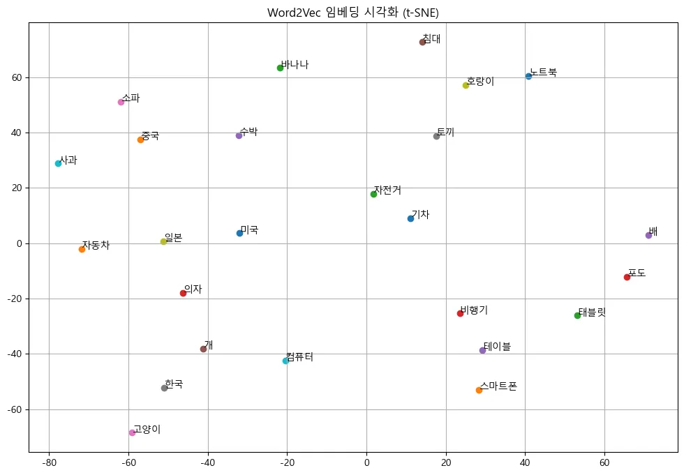
임베딩된 단어들을 시각화하였을 때 다음 이미지처럼 나왔는데, 학습 데이터가 굉장히 적어 적절한 임베딩이 되지 않았다고 생각하였다.
Annoy를 사용하여 단어 임베딩
from annoy import AnnoyIndex

dim = model.vector_size
annoy_index = AnnoyIndex(dim, 'angular')

# 모든 단어 벡터 추가
for i, word in enumerate(words):
    annoy_index.add_item(i, model.wv[word])
annoy_index.build(10)

# 유사한 단어 검색 (예: '사과')
target_word = '사과'
target_index = words.index(target_word)
similar_indices = annoy_index.get_nns_by_item(target_index, 5)

print(f"'{target_word}'와 유사한 단어:")
for i in similar_indices:
    print(words[i])
FAISS 대신 ANNOY를 사용하여 진행해보았고,
'사과'와 유사한 단어:
사과
일본
자전거
소파
중국
이 또한 적절하지 않음을 확인할 수 있었다.
나무위키 파일로 학습하기
from datasets import load_dataset

# Hugging Face에서 나무위키 데이터셋 로드
dataset = load_dataset("heegyu/namuwiki-extracted")
documents = dataset["train"].select(range(1000))  # 처음 1000개 문서만 사용 (속도 고려)
print(documents[0])
학습데이터가 적은 문제점을 해결하기 위하여 Hugging Face에서 제공하는 나무위키 데이터셋을 불러와 학습하고자 하였다.
시간이 오래 걸리는 관계 상 100개, 1000개, 3000개의 문서를 비교군으로 사용하였다.
import re
import kss
from tqdm import tqdm

def simple_tokenize(text):
    text = re.sub(r"[^\uAC00-\uD7A3\s]", "", text)
    return text.strip().split()

tokenized_sentences = []
for doc in tqdm(documents, desc="문장 분리 및 토큰화"):
    try:
        if not doc["text"].strip():
            continue
        sentences = kss.split_sentences(doc["text"])
        for sent in sentences:
            tokens = simple_tokenize(sent)
            if len(tokens) >= 1:
                tokenized_sentences.append(tokens)
    except Exception as e:
        continue
기본적으로 형태소를 기준으로 나눌 수는 없어 조사는 제외시키지 못하였고, 단순히 띄어쓰기를 기준으로 단어를 구분하였다.
from gensim.models import Word2Vec

model = Word2Vec(
    sentences=tokenized_sentences,
    vector_size=200,
    window=5,
    min_count=5,
    workers=4,
    sg=1,
    epochs=5
)
구분한 단어를 기준으로 모델을 학습시켜 단어 임베딩을 진행하였다.
print(model.wv.most_similar("한국"))다음과 같이 단어를 입력하고 입력된 단어를 기반으로 유사한 단어를 출력하도록 유도하였다.
1. 100개의 문서 만을 학습한 경우
[('신체', 0.9989925622940063), ('일부터', 0.998943030834198), ('앨범', 0.9982248544692993), ('게임', 0.9980660080909729), ('상대로', 0.9975945353507996), ('일에', 0.9973501563072205), ('기록했으나', 0.9973440170288086), ('북미', 0.9972758293151855), ('에서', 0.9972389340400696), ('첫', 0.9970090389251709)]
2. 1000개의 문서 만을 학습한 경우
[('중국', 0.7050928473472595), ('일본', 0.6985045075416565), ('대한민국', 0.6862316131591797), ('정식', 0.6725090742111206), ('아프리카', 0.6644840836524963), ('공식', 0.656909704208374), ('홍콩', 0.639904797077179), ('텔레비전', 0.6321231126785278), ('미', 0.6287841796875), ('일본에서', 0.6239179968833923)]
3. 3000개의 문서로 학습한 경우
[('대한민국', 0.5823025703430176), ('국내', 0.5639891624450684), ('중국', 0.5514899492263794), ('그룹', 0.5409524440765381), ('일본', 0.5325442552566528), ('대만', 0.505932092666626), ('아이돌', 0.49861907958984375), ('중국의', 0.49011966586112976), ('국적의', 0.4735112488269806), ('인기', 0.471205472946167)]
위와 같이 문서의 양이 늘어났을 때, 출력되는 단어의 종류가 육안으로도 향상됨을 확인할 수 있었다.
학습된 모델로 시각화
위의 나무위키를 통해서 학습된 모델을 바탕으로 위의 sentences 를 다시 시각화해보았다.
# 시각화할 단어 리스트
visual_words = [
    "사과", "바나나", "포도", "수박",
    "개", "고양이", "토끼", "호랑이",
    "컴퓨터", "노트북", "스마트폰", "태블릿",
    "의자", "테이블", "침대", "소파",
    "한국", "일본", "중국", "미국"
]
import numpy as np
valid_words = []
vectors = []
for word in visual_words:
if word in model.wv:
valid_words.append(word)
vectors.append(model.wv[word])
else:
print(f"⚠️ '{word}' 단어는 어휘 사전에 없습니다.")
vectors = np.array(vectors)앞서 말했던 학습데이터에 없던 데이터를 확인하고 제거하는 방식으로 시각화를 진행하였다.
1000개의 데이터셋을 활용한 경우에는 다음과 같이 존재하지 않는 단어도 존재했지만,
⚠️ '포도' 단어는 어휘 사전에 없습니다.
⚠️ '노트북' 단어는 어휘 사전에 없습니다.
⚠️ '태블릿' 단어는 어휘 사전에 없습니다.
⚠️ '소파' 단어는 어휘 사전에 없습니다.
3000개의 문서를 활용한 경우 학습데이터에서 제거되는 데이터는 존재하지 않았다. 즉, 모든 데이터를 시각화할 수 있었다.
from sklearn.manifold import TSNE
import matplotlib.pyplot as plt
import matplotlib.font_manager as fm
import platform

# t-SNE 차원 축소
tsne = TSNE(n_components=2, random_state=42, perplexity=5)
reduced = tsne.fit_transform(vectors)

# 한글 폰트 설정
if platform.system() == 'Windows':
    font_path = "C:/Windows/Fonts/malgun.ttf"
elif platform.system() == 'Darwin':
    font_path = "/System/Library/Fonts/AppleGothic.ttf"
else:
    font_path = "/usr/share/fonts/truetype/nanum/NanumGothic.ttf"

font_name = fm.FontProperties(fname=font_path).get_name()
plt.rc("font", family=font_name)
plt.rcParams["axes.unicode_minus"] = False

# 시각화
plt.figure(figsize=(10, 7))
for i, word in enumerate(valid_words):
    plt.scatter(reduced[i, 0], reduced[i, 1])
    plt.annotate(word, (reduced[i, 0], reduced[i, 1]))
plt.title("지정 단어 Word2Vec 시각화 (t-SNE)")
plt.grid(True)
plt.show()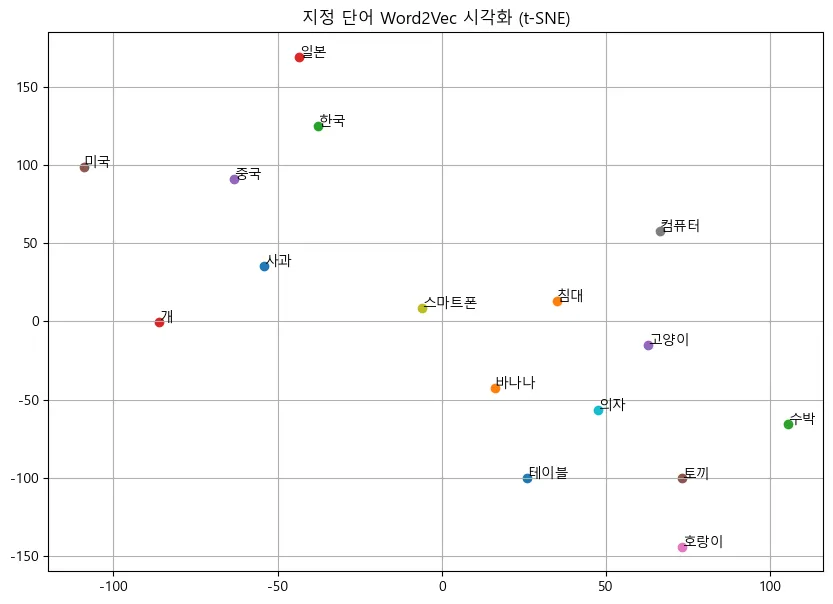
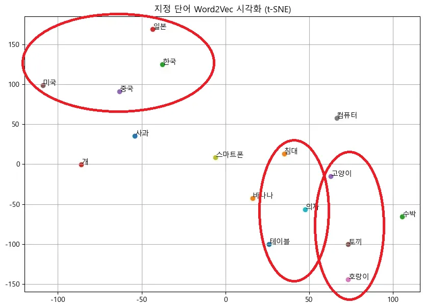
비교 및 정리
- 5개의 데이터로 학습한 모델의 경우
비슷한 종류의 데이터끼리 흩어져 있음을 확인할 수 있다.
- 나무위키를 통해 1000개의 데이터로 학습한 모델의 경우
많은 향상을 이루어내지는 못했지만, 어느 정도 향상된 결과가 나옴을 확인할 수 있었다.
- 나무위키 3000개의 문서로 학습한 모델의 경우
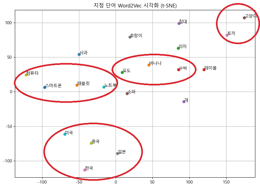
육안으로도 1000개의 데이터를 통해 학습한 모델보다 3000개의 데이터를 활용한 모델이 더 잘 구분됨을 확인할 수 있었다.
| 모델 | 군집수 |
|---|---|
| 5개로 학습 | X |
| 1000개로 학습 | 3개 정도의 군집 |
| 3000개로 학습 | 4~5개 정도의 군집 |
한계
- 학습 데이터 부족
KeyError: "Key '인공지능' not present in vocabulary”
위의 코드는 모델에 “인공지능”이라는 키워드를 넣었을 때, 출력되는 단어였다. 위의 에러처럼 만약 학습시킨 문서에 해당 단어가 없다면 유사도를 출력할 수 없는 문제가 존재했다.
- 조사 처리 X
또한, 위의 출력 결과들을 확인하면 조사를 제거하지 않아 “일본”과 “알본에서”가 각각 출력되는 것을 확인할 수 있다.
만약 모델의 성능을 향상시키기 위해서는 조사를 처리하는 방식으로 형태소를 구분해 모델 성능을 향상시킬 수 있을 것이라고 생각된다.
한계의 보완 - 조사 처리
KoNLPy란?
- 한국어 형태소 분석을 위한 파이썬 라이브러리이다.
- 여러 형태소 분석기(예: Okt, Kkma, Hannanum, Mecab 등)를 파이썬에서 사용할 수 있도록 래핑할 수 있다.
그 중에서, Okt는 "Open Korea Text"를 사용하여 품사를 태깅해 명사와 동사만을 추출하여 단어 임베딩을 진행하였다.
import re
import kss
from konlpy.tag import Okt
from tqdm import tqdm

okt = Okt()

def extract_nouns_verbs(text):
    text = re.sub(r"[^\uAC00-\uD7A3\s]", "", text)  # 한글과 공백만 유지
    return [word for word, pos in okt.pos(text) if pos in ['Noun', 'Verb']]

tokenized_sentences = []

for doc in tqdm(documents, desc="문장 분리 및 품사 필터링"):
    try:
        if not doc["text"].strip():
            continue
        sentences = kss.split_sentences(doc["text"])
        for sent in sentences:
            tokens = extract_nouns_verbs(sent)
            if len(tokens) >= 1:
                tokenized_sentences.append(tokens)
    except:
continueprint(model.wv.most_similar("수학"))[('과목', 0.9074293375015259), ('응시', 0.8836804032325745), ('성적표', 0.8830194473266602), ('수생', 0.8793541789054871), ('시험', 0.8571914434432983), ('국어', 0.853074848651886), ('한국사', 0.8445228338241577), ('고과', 0.8427404761314392), ('학년', 0.8421928882598877), ('대학', 0.8208978176116943)]
성능이 향상됨을 확인할 수 있으며, 조사 또한 제거되었다.