🎲[AI] Stochastic Gradient Descent

해당 글은 FastCampus - '[skill-up] 처음부터 시작하는 딥러닝 유치원 강의를 듣고,
추가 학습한 내용을 덧붙여 작성하였습니다.

---

1. Gradient Descent vs Stochastic Gradient Descent

1.1 Gradient Descent (GD)

• $Loss= {1 \over N} * \sum_{i=1}^{N} (y_i - ŷ_i)^2$
• 전체 데이터셋의 Loss를 기반으로 파라미터 1회 업데이트
• 정확한 gradient 방향이지만 계산량이 매우 큼
• 실제로 N의 크기가 매우 크면 OOM 에러 날 것

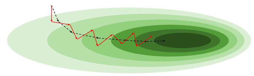
1.2 Stochastic Gradient Descent (SGD)

• $Loss= {1 \over K} * \sum_{i=1}^{K} (y_i - ŷ_i)^2$
• 무작위로 선택된 K개의 샘플(mini-batch)에 대한 Loss로 파라미터를 여러번 업데이트
• 계산량이 작고 빠르지만, gradient는 noisy할 수 있음
• Stochastic(확률론적) ↔ Deterministic(결정론적)

1.3 SGD의 특성

• 각 미니배치 gradient는 전체 gradient와 다를 수 있으나, 기대값은 같음
  
• 미니배치가 작을수록 gradient의 분산이 커짐
• 이로 인해 local minima에서 탈출 가능성이 생기기도 함
• 반면 batch size가 크면 빠른 수렴 가능
• Pytorch에서 optim.SGD는 전체 데이터를 넣으면 GD처럼 작동하고, 미니배치를 넣으면 SGD 또는 Mini-batch GD처럼 작동

---

2. Epoch과 Iteration

2.1 Epoch

• 전체 데이터셋이 한 번 학습된 횟수 (미니배치를 비복원추출 시 모든 데이터를 학습한 경우)
• 모든 데이터셋의 샘플들이 forward & backward 된 횟수
• Epoch의 시작에 데이터셋을 random shuffling 해준 후, 미니 배치로 나눔

2.2 Iteration

• 한 미니배치가 학습된 횟수

2.3 총 업데이트 횟수

• 파라미터 전체 업데이트 횟수 = $n\_epochs \ X \ n\_iterations$
• 이중 for loop이 만들어짐

for epoch_idx in n_epochs:
	for iteration_idx in n_iterations:
    ~~

---

3. Batch Size에 따른 특성

3.1 Full Batch (= 전체 데이터셋 크기)

• 전체 데이터의 분포를 잘 반영한 gradient
• 매우 정확하지만 계산량이 많고 업데이트 횟수가 적음

3.2 Small Batch

• 편향된 gradient를 가질 수 있음
• 오히려 local minima 탈출을 도울 수 있음
• 너무 작으면 gradient가 noisy하여 수렴이 어려워질 수 있음

3.3 적당한 Batch size는?

• $2^n$ 크기의 적절한 batchsize를 사용한다
  e.g. 64, 128, 256
• 근데 요즘은 GPU 하드웨어(메모리)의 성능이 뒷받쳐주기 때문에 큰 batch_size를 가져가기도 한다
  e.g. 2048, 4096 ,...

---

4. Pytorch 실습 코드

import pandas as pd
import seaborn as sns
import matplotlib.pyplot as plt
from sklearn.preprocessing import StandardScaler
import torch
import torch.nn as nn
import torch.nn.functional as F
import torch.optim as optim
from sklearn.datasets import fetch_california_housing

california = fetch_california_housing()

df = pd.DataFrame(california.data, columns=california.feature_names)
df["Target"] = california.target
# df.tail()

# sns.pairplot(df.sample(1000))
# plt.show()

scaler = StandardScaler()
scaler.fit(df.values[:, :-1])
df.values[:, :-1] = scaler.transform(df.values[:, :-1])

# sns.pairplot(df.sample(1000))
# plt.show()

data = torch.from_numpy(df.values).float()

print(data.shape)

x = data[:, :-1]
y = data[:, -1:]

print(x.shape, y.shape)

n_epochs = 4000
batch_size = 128
print_interval = 200
learning_rate = 1e-5

model = nn.Sequential(
    nn.Linear(x.size(-1), 10),
    nn.LeakyReLU(),
    nn.Linear(10, 9),
    nn.LeakyReLU(),
    nn.Linear(9, 8),
    nn.LeakyReLU(),
    nn.Linear(8, 7),
    nn.LeakyReLU(),
    nn.Linear(7, 6),
    nn.LeakyReLU(),
    nn.Linear(6, 5),
    nn.LeakyReLU(),    
    nn.Linear(5, 4),
    nn.LeakyReLU(),
    nn.Linear(4, 3),
    nn.LeakyReLU(),
    nn.Linear(3, y.size(-1)),
)

print(model)

optimizer = optim.SGD(model.parameters(), lr=learning_rate)

# |x| = (total_size, input_dim)
# |y| = (total_size, output_dim)

for i in range(n_epochs):
    #  the index to feed-forward.
    indices = torch.randperm(x.size(0)) # Shuffle
    x_ = torch.index_select(x, dim=0, index=indices) # x와 y indices 동일하게 써야 함
    y_ = torch.index_select(y, dim=0, index=indices)
    
    x_ = x_.split(batch_size, dim=0)
    y_ = y_.split(batch_size, dim=0)
    # |x_[i]| = (batch_size, input_dim)
    # |y_[i]| = (batch_size, output_dim)
    
    y_hat = []
    total_loss = 0
    
    for x_i, y_i in zip(x_, y_):
        # |x_i| = |x_[i]|
        # |y_i| = |y_[i]|
        y_hat_i = model(x_i)
        loss = F.mse_loss(y_hat_i, y_i)

        optimizer.zero_grad()
        loss.backward()

        optimizer.step()
        
        total_loss += float(loss) # Gradient graph 끊어짐 → float로 변환해서 memory leak 방지
        y_hat += [y_hat_i]

    total_loss = total_loss / len(x_)
    if (i + 1) % print_interval == 0:
        print('Epoch %d: loss=%.4e' % (i + 1, total_loss))
    
y_hat = torch.cat(y_hat, dim=0)
y = torch.cat(y_, dim=0)
# |y_hat| = (total_size, output_dim)
# |y| = (total_size, output_dim)

df = pd.DataFrame(torch.cat([y, y_hat], dim=1).detach().numpy(),
                  columns=["y", "y_hat"])

sns.pairplot(df, height=5)
plt.show()

---