Naive Bayes

나이브 베이즈 (Naive Bayes)

1. 나이브 베이즈

• 나이브 베이즈(Naive Bayes)는 확률 기반의 분류 알고리즘
• 베이즈 정리(Bayes' Theorem)를 기반으로 동작
• 각 특징(feature)이 서로 독립이라는 "나이브(naive, 순진한)" 가정을
• -> 계산이 빠르고 간단한 모델

📌 특징

• 확률 모델(Probabilistic Model) → 결과를 확률로 해석 가능
• 빠르고 효율적 → 데이터 크기가 커도 빠르게 학습
• 독립 가정(Independence Assumption) → 일부 데이터셋에서는 제한적

---

2. 베이즈 정리(Bayes' Theorem)

나이브 베이즈는 베이즈 정리를 기반:

✅ 설명

• $P(A | B)$: 사후 확률(Posterior Probability) → B가 주어졌을 때 A가 발생할 확률
• $P(B | A)$: 가능도(Likelihood) → A가 발생했을 때 B가 발생할 확률
• $P(A)$: 사전 확률(Prior Probability) → A가 발생할 확률
• $P(B)$ 정규화 상수(Evidence) → 모든 가능한 A에 대한 확률의 총합

📝 쉽게 정리하면

사후 확률(Posterior) = 사전 확률(Prior) × 가능도(Likelihood) ÷ 증거(Evidence)

---

3. 예제 (날씨와 비의 관계)

1️⃣ 문제 정의

• 날씨(맑음, 흐림)에 따라 비가 올 확률을 예측

2️⃣ 데이터 테이블

날씨	비 옴 (☔)	비 안 옴	합계
맑은 날 ☀	3	7	10
흐린 날 ☁	5	5	10
합계	8	12	20

3️⃣ 확률 계산

사전 확률 (Prior Probability)

• $P(\text{맑은 날}) = \frac{10}{20} = 0.5$
• $P(\text{비}) = \frac{8}{20} = 0.4$

가능도 (Likelihood) - 특정 날씨일 때 비가 올 확률

• $P(\text{맑은 날 | 비}) = \frac{3}{8} = 0.375$

증거 (Evidence)

• $P(\text{비}) = \frac{8}{20} = 0.4$

사후 확률 (Posterior Probability)

• $P(\text{비 | 맑은 날}) = \frac{P(\text{맑은 날} | \text{비}) P(\text{비})}{P(\text{맑은 날})}$
• $P(\text{비 | 맑은 날}) = \frac{(3/8) \times (0.4)}{0.5} = \frac{0.15}{0.5} = 0.35$

즉, 날씨가 맑을 때 비가 올 확률은 35%

---

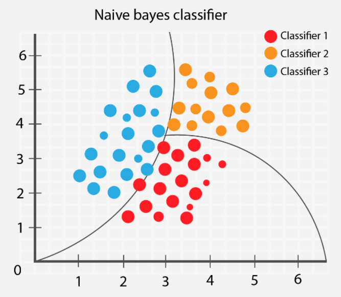
4. 나이브 베이즈의 종류

나이브 베이즈는 데이터의 특성에 따라 여러 변형이 있습니다.

1️⃣ 가우시안 나이브 베이즈 (Gaussian Naive Bayes)

• 특징이 연속형(Continuous Data)일 때 사용
• 특징이 정규 분포(Gaussian Distribution)를 따른다고 가정
• 확률 밀도 함수(PDF) 사용:

📌 사용 예시: 키, 몸무게, 온도 등 연속형 데이터 분류

---

2️⃣ 멀티노미얼 나이브 베이즈 (Multinomial Naive Bayes)

• 특징이 이산형(Discrete Data)일 때 사용
• 단어 등장 횟수 기반의 문서 분류에 적합 (e.g., 텍스트 분류)

📌 사용 예시: 이메일 스팸 분류, 뉴스 카테고리 분류

---

3️⃣ 베르누이 나이브 베이즈 (Bernoulli Naive Bayes)

• 특징이 0 또는 1(이진 값)을 가질 때 사용
• 특정 단어가 존재하는지 여부(예: 단어가 등장하면 1, 없으면 0)

📌 사용 예시: 텍스트 분류(문서에 특정 단어가 있는지 없는지)

---

5. 나이브 베이즈 구현 (Python 예제)

from sklearn.naive_bayes import GaussianNB
from sklearn.model_selection import train_test_split
from sklearn.datasets import load_iris

# 데이터 불러오기
iris = load_iris()
X_train, X_test, y_train, y_test = train_test_split(iris.data, iris.target, test_size=0.2, random_state=42)

# 가우시안 나이브 베이즈 모델 생성 및 학습
gnb = GaussianNB()
gnb.fit(X_train, y_train)

# 예측 및 평가
accuracy = gnb.score(X_test, y_test)
print(f'Accuracy: {accuracy:.2f}')

---

6. 나이브 베이즈의 장단점

✅ 장점

• 계산량이 적어 빠르고 효율적
• 적은 데이터로도 학습 가능
• 확률 기반 예측 → 결과 해석 가능
• 텍스트 분류 등 특정 도메인에서 뛰어난 성능

❌ 단점

• 독립 가정이 현실적이지 않을 수 있음 (특징 간의 상관관계를 고려하지 않음)
• 연속형 데이터에서 정규 분포를 따르지 않으면 성능 저하 가능

---

7. 결론

• 나이브 베이즈는 빠르고 가벼운 분류 모델로, 특히 텍스트 분류(스팸 필터링, 감성 분석)에서 많이 사용
• 독립 가정의 한계 존재, 데이터가 적어도 높은 성능을 보일 수 있는 알고리즘

---

python

가우시안 나이브 베이즈

1. 데이터 준비

from sklearn.datasets import load_iris
from sklearn.model_selection import train_test_split, GridSearchCV
from sklearn.naive_bayes import GaussianNB
from sklearn.metrics import accuracy_score
import numpy as np
import pandas as pd
import matplotlib.pyplot as plt
import seaborn as sns

data = load_iris()
X = data.data  # 특성 데이터
y = data.target  # 라벨 데이터
feature = data.feature_names  # 특성 이름 리스트

• load_iris() : 사이킷런에서 제공하는 붓꽃(Iris) 데이터셋 로드
• X : 입력 변수 (꽃잎과 꽃받침의 길이 및 너비)
• y : 타겟 변수 (0: Setosa, 1: Versicolor, 2: Virginica)
• feature : 각 피처의 이름

---

2. 하이퍼파라미터 최적화 (GridSearchCV)

param_grid = {'var_smoothing': np.logspace(0, -9, num=100)}
gnb = GaussianNB()
grid_search = GridSearchCV(gnb, param_grid, cv=5, scoring='accuracy')
grid_search.fit(X, y)

• var_smoothing: 가우시안 나이브 베이즈의 분산 스무딩(variance smoothing) 계수를 최적화하는 하이퍼파라미터
  • np.logspace(0, -9, num=100): $10^0$에서 $10^{-9}$까지 100개의 값 생성
  • 분산을 조절하여 모델의 일반화 성능을 개선하는 역할
• GridSearchCV(gnb, param_grid, cv=5, scoring='accuracy')
  • 5-폴드 교차 검증을 사용하여 최적의 var_smoothing 찾기
  • accuracy(정확도)를 기준으로 성능 평가

---

3. 최적 모델 학습 및 평가

best_gnb = grid_search.best_estimator_  # 최적 모델
y_pred = best_gnb.predict(X)  # 모델 예측값
accuracy = accuracy_score(y, y_pred)  # 정확도 계산

print('Best estimates found', grid_search.best_params_)
print(f'Model Accuracy : {accuracy : .4f}')

• grid_search.best_estimator_ : 최적의 하이퍼파라미터를 적용한 가우시안 나이브 베이즈 모델
• accuracy_score(y, y_pred): 훈련 데이터에 대한 정확도 계산

주의점

• 훈련 데이터(X)에 대해 평가하므로, 과적합(overfitting) 가능성이 존재함.
• 실제 모델 성능을 평가하려면 train_test_split()을 사용하여 훈련/테스트 데이터로 나눈 후 검증해야 함.

---

4. 피처 중요도 계산 및 시각화

feature_importance = 1 / (best_gnb.var_).mean(axis=0)
importance_df = pd.DataFrame({'Feature': feature, 'Importance': feature_importance})

importance_df = importance_df.sort_values(by='Importance', ascending=False)

plt.figure(figsize=(10, 10))
sns.barplot(x="Importance", y="Feature", data=importance_df)
plt.title("Feature Importance (GaussianNB)")
plt.xlabel("Importance Score (1/var)")
plt.ylabel("Features")
plt.show()

out:

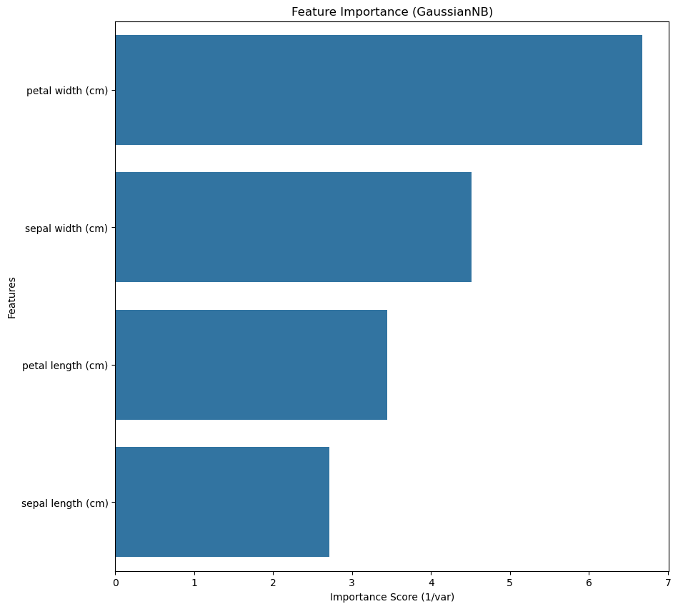
피처 중요도 계산

• 나이브 베이즈 모델은 결정 트리처럼 명시적인 특성 중요도를 제공하지 않음.
• 대신 각 피처의 분산(variance)이 작을수록 더 중요한 특성으로 간주할 수 있음.
  • best_gnb.var_ : 가우시안 나이브 베이즈 모델의 각 피처별 분산
  • 1 / (best_gnb.var_).mean(axis=0) : 분산의 역수를 이용해 특성 중요도를 정의
    • 분산이 작을수록 가우시안 확률 분포가 더 좁아지며, 결정에 더 큰 영향을 미침.

시각화

• importance_df.sort_values(by='Importance', ascending=False): 중요도가 높은 순서로 정렬
• sns.barplot(x="Importance", y="Feature", data=importance_df): 피처 중요도를 바 플롯으로 시각화
• 높은 중요도를 가진 피처가 모델 예측에 더 큰 영향을 미치는 특성이라고 볼 수 있음.

---

코드 전체 요약

1. 아이리스 데이터셋 로드
2. GridSearchCV를 사용해 var_smoothing 최적화
3. 최적 모델로 훈련 데이터 예측 및 정확도 평가
4. 가우시안 나이브 베이즈 모델에서 피처 중요도를 계산하여 시각화

---

추가 개선 포인트

• 데이터를 훈련/테스트 세트로 분리하여 일반화 성능 평가

  X_train, X_test, y_train, y_test = train_test_split(X, y, test_size=0.2, random_state=42)
  grid_search.fit(X_train, y_train)
  best_gnb = grid_search.best_estimator_
  y_test_pred = best_gnb.predict(X_test)
  test_accuracy = accuracy_score(y_test, y_test_pred)
  print(f'Model Test Accuracy: {test_accuracy:.4f}')

  • test_size=0.2 : 20% 데이터를 테스트용으로 사용
  • 일반적으로 훈련 데이터 정확도가 높고 테스트 데이터 정확도가 낮으면 과적합 가능성이 있음.