1. 로지스틱 회귀란?

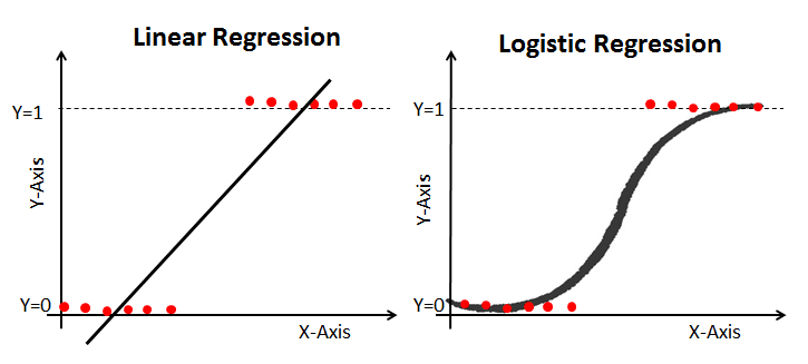
• 이진 분류(Binary Classification)를 수행하는 지도 학습(Supervised Learning) 알고리즘
• 일반적인 선형 회귀(Linear Regression)를 기반으로
  • 결과를 확률값(0~1 사이)로 변환하여 분류 문제에 적용

📌 특징

• 입력 데이터의 선형 결합을 기반으로 확률을 예측
• 시그모이드(Sigmoid) 함수를 사용하여 예측값을 0과 1 사이로 변환
• 손실 함수로 로그 손실(Binary Cross-Entropy) 사용

---

2. 로그의 특성과 로짓 변환 (Logit Transformation)

2-1 로그의 특성(Log Properties)

1. $\log(ab) = \log a + \log b$
2. $\log \frac{a}{b} = \log a - \log b$
3. $\log a^b = b \log a$

확률을 선형 회귀의 형태로 변환하는 데 유용

2-2 로짓 변환(Logit Function)

오즈비를 로그를 씌워서 선형회귀로 나타냄

로짓 함수(Logit function)의 정의:

여기서:

• $p$는 1이 될 확률 $P(y=1 | x)$
• $\frac{p}{1 - p}$는 오즈(odds)라고 불리며, 특정 사건이 발생할 확률과 발생하지 않을 확률의 비율을 나타냄

로지스틱 회귀에서는 확률 $p$를 선형 결합 형태로 나타냄

오즈의 로그(log-odds)는 선형 회귀 형태로 표현
로지스틱 함수(Logistic Function)를 사용하여 확률값으로 변환

로지스틱 회귀에서 오즈는 어떤 사건이 발생할 확률 대비 안 일어날 확률의 비율임. 승률(확률)이 높을수록 오즈도 커지는데, 로짓 변환(log-odds)하면 강자가 더 높은 값(불리한 패널티처럼 보이는 값)을 갖게 됨.

---

3. 로지스틱 함수(Logistic Function) 및 미분 특성

3-1 로지스틱 함수 (시그모이드 함수)

로지스틱 회귀는 시그모이드(Sigmoid) 함수를 사용하여 선형 결합 값을 확률값으로 변환

$z$: 선형 회귀의 결과값

이 함수는 $z$가 증가할수록 1에 가까워지고, 감소할수록 0에 가까워지는 특성

---

3-2 로지스틱 함수의 미분

로지스틱 회귀에서 경사 하강법(Gradient Descent)을 사용하여 최적의 가중치를 찾을 때, 로지스틱 함수의 미분 특성을 활용

시그모이드 함수 $h(z)$의 미분:

✅ 미분 특성의 활용

• 미분 결과가 다시 자신의 값과 1에서 뺀 값의 곱으로 나타남 → 계산이 간편
• 경사 하강법에서 업데이트하는 과정이 효율적으로 수행됨

---

4. 비용 함수 (Binary Cross-Entropy)

로지스틱 회귀는 MSE(평균제곱오차, Mean Squared Error) 대신 로그 손실(Binary Cross-Entropy, Log Loss)를 사용

✅ 이해하기 쉽게 풀어보면

• $y_i = 1$일 때 → 첫 번째 항 $\log h(z_i)$만 남음 (예측값이 1에 가까울수록 손실 감소)
• $y_i = 0$일 때 → 두 번째 항 $\log(1 - h(z_i))$만 남음 (예측값이 0에 가까울수록 손실 감소)

이 손실 함수를 경사 하강법(Gradient Descent)을 사용하여 최소화함.

---

5. 로지스틱 회귀의 장단점

✅ 장점

• 이해하기 쉽고 해석 가능한 모델
• 계산 비용이 낮아 빠르게 학습 가능
• 확률 기반 예측이 가능하여 의사 결정에 유용

❌ 단점

• 선형적으로 분리되지 않는 데이터에 한계
• 다중 분류(Multiclass Classification)에서는 소프트맥스 회귀(Softmax Regression) 필요
• 다양한 비선형 패턴을 학습하기 어려움

---

6. 로지스틱 회귀를 잘 활용하려면?

📌 특징 엔지니어링(Feature Engineering): 비선형 데이터의 경우 다항식 특징 추가
📌 정규화(Regularization): L1(Lasso), L2(Ridge) 정규화를 통해 과적합 방지
📌 확률적 해석: 예측 확률을 활용한 의사 결정 가능

---

로지스틱 회귀는 단순하지만 강력한 이진 분류 모델
특히 데이터가 선형적으로 구분될 때 좋은 성능을 발휘하며, 확률 기반의 해석이 가능

---

5. 로지스틱 회귀 구현 (Python 예제)

from sklearn.linear_model import LogisticRegression
from sklearn.model_selection import train_test_split
from sklearn.datasets import load_iris

# 데이터 불러오기
iris = load_iris()
X_train, X_test, y_train, y_test = train_test_split(iris.data, iris.target, test_size=0.2, random_state=42)

# 이진 분류를 위해 클래스 0과 1만 사용
X_train, X_test = X_train[y_train < 2], X_test[y_test < 2]
y_train, y_test = y_train[y_train < 2], y_test[y_test < 2]

# 로지스틱 회귀 모델 생성 및 학습
log_reg = LogisticRegression()
log_reg.fit(X_train, y_train)

# 예측 및 평가
accuracy = log_reg.score(X_test, y_test)
print(f'Accuracy: {accuracy:.2f}')

---

breast_cancer with Python

import data

import matplotlib.pyplot as plt
from sklearn.model_selection import train_test_split
from sklearn.datasets import load_breast_cancer

cancer = load_breast_cancer()

out:

[0 0 0 0 0 0 0 0 0 0 0 0 0 0 0 0 0 0 0 1 1 1 0 0 0 0 0 0 0 0 0 0 0 0 0 0 0
 1 0 0 0 0 0 0 0 0 1 0 1 1 1 1 1 0 0 1 0 0 1 1 1 1 0 1 0 0 1 1 1 1 0 1 0 0
 1 0 1 0 0 1 1 1 0 0 1 0 0 0 1 1 1 0 1 1 0 0 1 1 1 0 0 1 1 1 1 0 1 1 0 1 1
 1 1 1 1 1 1 0 0 0 1 0 0 1 1 1 0 0 1 0 1 0 0 1 0 0 1 1 0 1 1 0 1 1 1 1 0 1
   ..... ]

---

EDA

• find count one and 0

  sum(cancer.target) # target ==1
  len(cancer.target) - sum(cancer.target) # target ==0

  out:

  357
  212

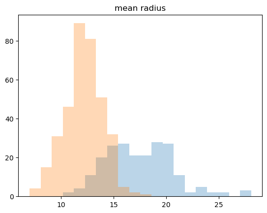
• histogram

  _,bins= np.histogram(cancer.data[:,0], bins=20)
  np.histogram(cancer.data[:,0],bins=20)
  plt.hist(malignant[:,0],bins=bins,alpha=0.3)
  plt.hist(benign[:,0], bins = bins, alpha=0.3)
  plt.title(cancer.feature_names[0])

  out:
  

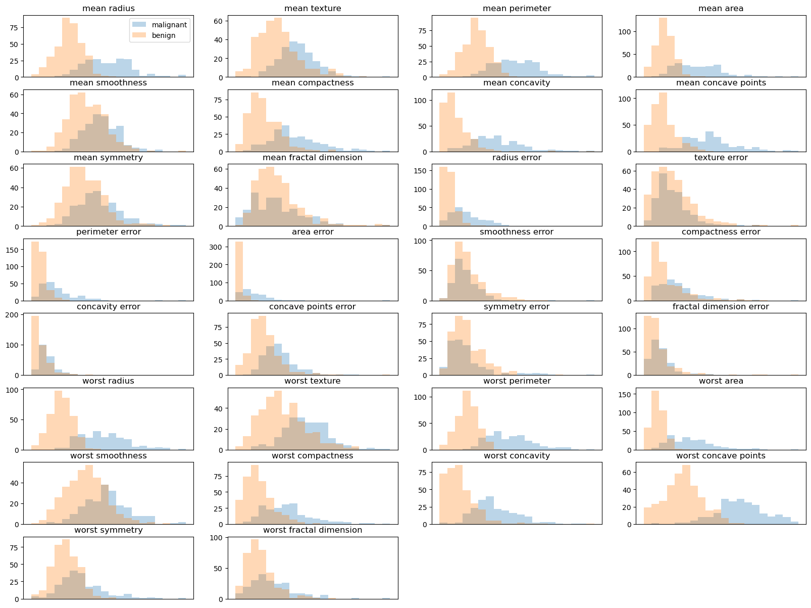
• draw whole feature

  plt.figure(figsize=(20,15)) #figsize:(float,float), default : rcParams['figure.figsize'](defulat:[6.4,4.8])
  for col in range(30):
     plt.subplot(8,4,col+1)
     _,bins = np.histogram(cancer.data[:,col],bins=20)
     plt.hist(malignant[:,col],bins=bins,alpha=0.3)
     plt.hist(benign[:,col], bins = bins, alpha=0.3)
     plt.title(cancer.feature_names[col])
     if col==0: plt.legend(cancer.target_names)
     plt.xticks([])
  plt.show()

  out:
  

---

Classification with LogisticRegression

from sklearn.linear_model import LogisticRegression

scores = []

for i in range(10):
    X_train, X_test, y_train, y_test = train_test_split(cancer.data, cancer.target, test_size = 0.2)
    model = LogisticRegression(max_iter=5000)
    
    model.fit(X_train,y_train)

    score = model.score(X_test, y_test)
    scores.append(score)
print("scores = ", scores)

out:

scores =  [0.9122807017543859, 0.9649122807017544, 0.9385964912280702, 0.9035087719298246, 0.9649122807017544, 0.9210526315789473, 0.956140350877193, 0.9473684210526315, 0.9649122807017544, 0.9649122807017544]

• Similar to the above code and kfold
• Wrong: may be redundant, may not get picked -> can't determine overfitting
• Let's use Kfold