Gradient Descent(복습)
우선 Gradient Descent를 복습해보자
임의의 함수 만들기
import numpy as np
import matplotlib.pyplot as plt
np.random.seed(42)
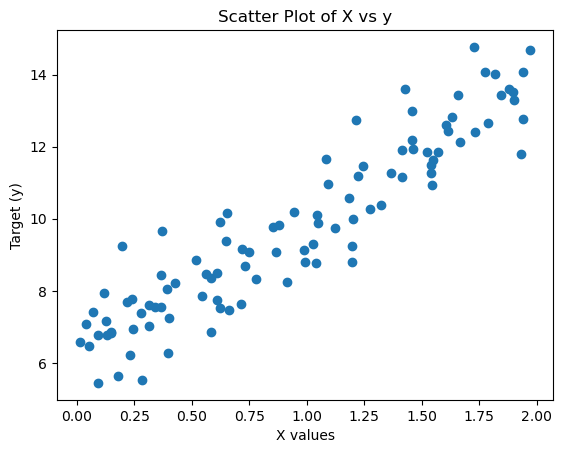
X = 2*np.random.rand(100,1)
y = 6+4*X+np.random.randn(100,1)
plt.scatter(X,y)
plt.xlabel("X values")
plt.ylabel("Target (y)")
plt.title("Scatter Plot of X vs y")
plt.show()out:
get_weight_updates
def get_weight_updates(w1,w0,X,y,learning_rate=0.01):
    N = len(y)
    y_pred = np.dot(X,w1) + w0
    diff = y-y_pred
    w1_update = -(learning_rate/N) * np.dot(X.T,diff)
    w0_update = -(learning_rate/N) * np.sum(diff)
    return w1_update, w0_update
get_cost
def get_cost(y,y_pred):
   N = len(y)
   cost = np.sum(np.square(y-y_pred))/N
   return cost
gradient_descent_steps
def gradient_descent_steps(X,y,learning_rate = 0.01, iters = 1000):
w0 = np.zeros((1,1))
w1 = np.zeros((1,1))
cost_list = []
w1_list = []
w0_list = []
for i in range(iters):
w1_update, w_0update = get_weight_updates(w1,w0,X,y,learning_rate)
w1 -= w1_update
w0 -= w_0update
w1_list.append(w1[0,0])
w0_list.append(w0[0,0])
y_pred = np.dot(X,w1) +w0
cost = get_cost(y,y_pred)
cost_list.append(cost)
if (i+1)%100 == 0:
print(f'Iteration {i+1}/{iters} - MSE : {cost:.4f}, w1:{w1[0,0]:.3f}, w0: {w0[0,0]:.3f}')
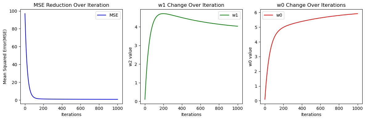
return w1, w0, cost_list, w1_list,w0_listMSE, W1, W0의 변화량 살펴보기
w1, w0, cost_list, w1_list, w0_list = gradient_descent_steps(X, y, iters=1000)
print("\n Optimized weights:")
print(f"w1:{w1[0,0]:.3f}, w0:{w0[0,0]:.3f}")
plt.figure(figsize=(12,4))

plt.subplot(1,3,1)
plt.plot(range(1,1001), cost_list, label='MSE', color = 'blue')
plt.xlabel("Iterations")
plt.ylabel("Mean Squared Error(MSE)")
plt.title("MSE Reduction Over Iteration")
plt.legend()

plt.subplot(1,3,2)
plt.plot(range(1,1001), w1_list, label='w1', color = 'green')
plt.xlabel("Iterations")
plt.ylabel("w2 value")
plt.title("w1 Change Over Iteration")
plt.legend()

plt.subplot(1,3,3)
plt.plot(range(1,1001), w0_list, label='w0', color = 'red')
plt.xlabel("Iterations")
plt.ylabel("w0 value")
plt.title("w0 Change Over Iterations")
plt.legend()

plt.tight_layout()
plt.show()
out:
집값 예측
데이터, 라이브러리 불러오기
import numpy as np
import pandas as pd
import matplotlib.pyplot as plt
import seaborn as sns

from sklearn.linear_model import LinearRegression
from sklearn.model_selection import train_test_split
from sklearn.metrics import mean_squared_error

df = pd.read_csv(r'C:/Users/user/LG/pythonVScode/regression/HousingData.csv')
boston_data = df.dropna(axis=0)
boston_data
out:
	CRIM	ZN	INDUS	CHAS	NOX	RM	AGE	DIS	RAD	TAX	PTRATIO	B	LSTAT	MEDV
0	0.00632	18.0	2.31	0.0	0.538	6.575	65.2	4.0900	1	296	15.3	396.90	4.98	24.0
1	0.02731	0.0	7.07	0.0	0.469	6.421	78.9	4.9671	2	242	17.8	396.90	9.14	21.6
2	0.02729	0.0	7.07	0.0	0.469	7.185	61.1	4.9671	2	242	17.8	392.83	4.03	34.7
3	0.03237	0.0	2.18	0.0	0.458	6.998	45.8	6.0622	3	222	18.7	394.63	2.94	33.4
5	0.02985	0.0	2.18	0.0	0.458	6.430	58.7	6.0622	3	222	18.7	394.12	5.21	28.7
...	...	...	...	...	...	...	...	...	...	...	...	...	...	...
499	0.17783	0.0	9.69	0.0	0.585	5.569	73.5	2.3999	6	391	19.2	395.77	15.10	17.5
500	0.22438	0.0	9.69	0.0	0.585	6.027	79.7	2.4982	6	391	19.2	396.90	14.33	16.8
502	0.04527	0.0	11.93	0.0	0.573	6.120	76.7	2.2875	1	273	21.0	396.90	9.08	20.6
503	0.06076	0.0	11.93	0.0	0.573	6.976	91.0	2.1675	1	273	21.0	396.90	5.64	23.9
504	0.10959	0.0	11.93	0.0	0.573	6.794	89.3	2.3889	1	273	21.0	393.45	6.48	22.0
EDA 분석
boston_data.info()out:
<class 'pandas.core.frame.DataFrame'>
Index: 394 entries, 0 to 504
Data columns (total 14 columns):
 #   Column   Non-Null Count  Dtype
---  ------   --------------  -----
 0   CRIM     394 non-null    float64
 1   ZN       394 non-null    float64
 2   INDUS    394 non-null    float64
 3   CHAS     394 non-null    float64
 4   NOX      394 non-null    float64
 5   RM       394 non-null    float64
 6   AGE      394 non-null    float64
 7   DIS      394 non-null    float64
 8   RAD      394 non-null    int64
 9   TAX      394 non-null    int64
 10  PTRATIO  394 non-null    float64
 11  B        394 non-null    float64
 12  LSTAT    394 non-null    float64
 13  MEDV     394 non-null    float64
dtypes: float64(12), int64(2)
memory usage: 46.2 KBboston_data.describe()
out:
	CRIM	ZN	INDUS	CHAS	NOX	RM	AGE	DIS	RAD	TAX	PTRATIO	B	LSTAT	MEDV
count	394.000000	394.000000	394.000000	394.000000	394.000000	394.000000	394.000000	394.000000	394.000000	394.000000	394.000000	394.000000	394.000000	394.000000
mean	3.690136	11.460660	11.000863	0.068528	0.553215	6.280015	68.932741	3.805268	9.403553	406.431472	18.537563	358.490939	12.769112	22.359645
std	9.202423	23.954082	6.908364	0.252971	0.113112	0.697985	27.888705	2.098571	8.633451	168.312419	2.166460	89.283295	7.308430	9.142979
min	0.006320	0.000000	0.460000	0.000000	0.389000	3.561000	2.900000	1.129600	1.000000	187.000000	12.600000	2.600000	1.730000	5.000000
25%	0.081955	0.000000	5.130000	0.000000	0.453000	5.879250	45.475000	2.110100	4.000000	280.250000	17.400000	376.707500	7.125000	16.800000
50%	0.268880	0.000000	8.560000	0.000000	0.538000	6.201500	77.700000	3.199200	5.000000	330.000000	19.100000	392.190000	11.300000	21.050000
75%	3.435973	12.500000	18.100000	0.000000	0.624000	6.605500	94.250000	5.116700	24.000000	666.000000	20.200000	396.900000	17.117500	25.000000
max	88.976200	100.000000	27.740000	1.000000	0.871000	8.780000	100.000000	12.126500	24.000000	711.000000	22.000000	396.900000	37.970000	50.000000
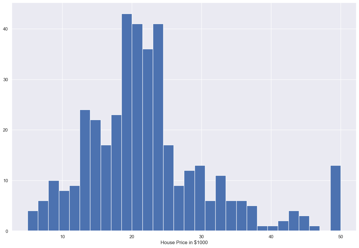
가격에 대한 집 분포
sns.set(rc={'figure.figsize':(15,10)})
plt.hist(boston_data['MEDV'],bins=30)
plt.xlabel("House Price in $1000")
plt.show()
out:
공분산 정도 살펴보기
correlation_matrix = boston_data.corr().round(2)
sns.heatmap(data=correlation_matrix, annot=True)
out:
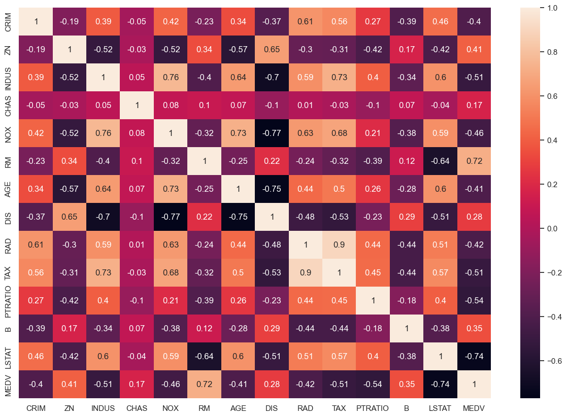
- 상관계수가 높은 LSTAT, RM선별
- 상관계수가 낮은 DIS 선별
가격에 대한 분포 살펴보기 1
plt.figure(figsize=(20,5))
features = ['LSTAT', 'RM', 'DIS']
target = boston_data['MEDV']

for i, col in enumerate(features):
    plt.subplot(1,len(features), i+1)
    x=boston_data[col]
    y= target
    plt.scatter(x,y, marker='o', color = '#e35f62')
    plt.title("Variation in House prices")
    plt.xlabel(col)
    plt.ylabel('"House prices in $1000"')
out:

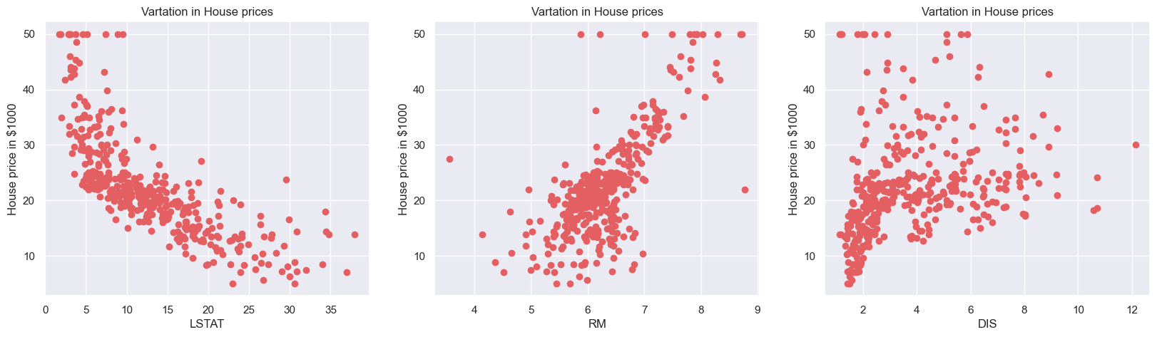
가격에 대한 분포 살펴보기 2
plt.figure(figsize=(20,5))
features = ['LSTAT', 'RM', 'DIS'] #for 안에 subplot -> subplots로
fig,axs = plt.subplots(1,len(features), figsize=(20,5))
for i,col in enumerate(features):
    x = boston_data[col]
    y = boston_data['MEDV']
    axs[i].scatter(x,y,marker='o', color = '#e35f62')
    axs[i].set_title("Vartation in House prices")
    axs[i].set_xlabel(col)
    axs[i].set_ylabel("House price in $1000")

plt.show()
out: :
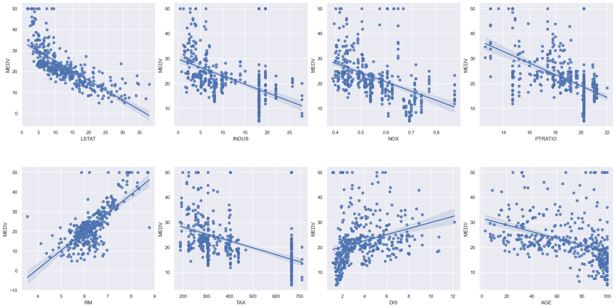
선형회귀plot (regplot) 그려보기
column_sels = ['LSTAT','INDUS','NOX','PTRATIO','RM','TAX','DIS','AGE']
x = boston_data.loc[:,column_sels]
y = boston_data['MEDV']
fig, axs = plt.subplots(ncols=4, nrows=2, figsize=(20, 10))
index = 0
axs = axs.flatten()
for i, k in enumerate(column_sels):
    sns.regplot(y=y, x=x[k], ax=axs[i])
plt.tight_layout(pad=0.4, w_pad=0.5, h_pad=5.0)
out:
ROOM만 빼서 선형회귀 하기
전처리 하기
x_rooms = boston_data['RM']
y_prices = boston_data['MEDV']
##scikit-learn은 항상 2차원을 받아들인다.

##2차원으로 만들어 주자
x_rooms = np.array(x_rooms).reshape(-1,1)
y_prices = np.array(y_prices).reshape(-1,1)

X_train,X_test,y_train,y_test = train_test_split(x_rooms,y_prices,test_size=0.2,random_state=5)
선형 회귀
reg_1 = LinearRegression()
reg_1.fit(X_train,y_train)

y_test_predict = reg_1.predict(X_test)
rmse = (np.sqrt(mean_squared_error(y_test, y_test_predict)))
r2 = round(reg_1.score(X_test,y_test),2)

print("The model performance for training set")
print("---------------------------------------")
print('RMSE is {}'.format(rmse))
print('R2 score is {}'.format(r2))
print('\n')
out:
The model performance for training set
---------------------------------------
RMSE is 6.417885493331466
R2 score is 0.49
시각화
prediction_space = np.linspace(min(x_rooms),max(x_rooms)).reshape(-1,1)
plt.scatter(x_rooms, y_prices)
plt.plot(prediction_space, reg_1.predict(prediction_space),color='black', linewidth=3)
plt.ylabel('value of house/1000($)')
plt.xlabel('number of rooms')
plt.show()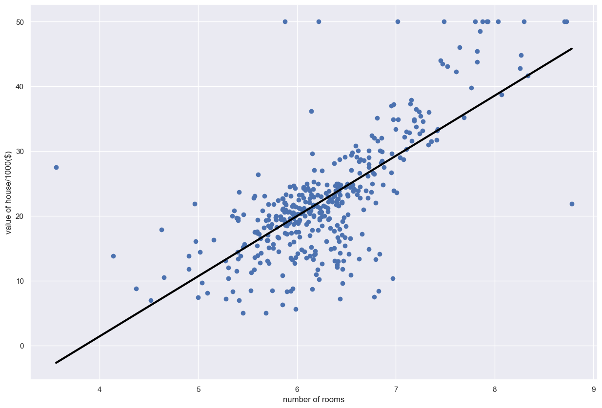
모든 변수 넣고 진행
y= bos.pop('MEDV')
X= bos
X_train,X_test,y_train,y_test = train_test_split(X,y,test_size=0.2,random_state=5)


reg_all = LinearRegression()
reg_all.fit(X_train,y_train)

y_test_predict = reg_all.predict(X_test)
rmse = (np.sqrt(mean_squared_error(y_test, y_test_predict)))
r2 = round(reg_all.score(X_test,y_test),2)

print("The model performance for training set")
print("---------------------------------------")
print('RMSE is {}'.format(rmse))
print('R2 score is {}'.format(r2))
print('\n')
K-fol cross validation
데이터 불러오기
import numpy as np
import pandas as pd
import matplotlib.pyplot as plt
import seaborn as sns

from sklearn.linear_model import LinearRegression
from sklearn.model_selection import train_test_split, cross_val_score
from sklearn.metrics import mean_squared_error, r2_score

df = pd.read_csv(r'C:/Users/user/LG/pythonVScode/regression/HousingData.csv')
boston_data = df.dropna(axis=0)
boston_data
out:
	CRIM	ZN	INDUS	CHAS	NOX	RM	AGE	DIS	RAD	TAX	PTRATIO	B	LSTAT	MEDV
0	0.00632	18.0	2.31	0.0	0.538	6.575	65.2	4.0900	1	296	15.3	396.90	4.98	24.0
1	0.02731	0.0	7.07	0.0	0.469	6.421	78.9	4.9671	2	242	17.8	396.90	9.14	21.6
2	0.02729	0.0	7.07	0.0	0.469	7.185	61.1	4.9671	2	242	17.8	392.83	4.03	34.7
3	0.03237	0.0	2.18	0.0	0.458	6.998	45.8	6.0622	3	222	18.7	394.63	2.94	33.4
5	0.02985	0.0	2.18	0.0	0.458	6.430	58.7	6.0622	3	222	18.7	394.12	5.21	28.7
...	...	...	...	...	...	...	...	...	...	...	...	...	...	...
499	0.17783	0.0	9.69	0.0	0.585	5.569	73.5	2.3999	6	391	19.2	395.77	15.10	17.5
500	0.22438	0.0	9.69	0.0	0.585	6.027	79.7	2.4982	6	391	19.2	396.90	14.33	16.8
502	0.04527	0.0	11.93	0.0	0.573	6.120	76.7	2.2875	1	273	21.0	396.90	9.08	20.6
503	0.06076	0.0	11.93	0.0	0.573	6.976	91.0	2.1675	1	273	21.0	396.90	5.64	23.9
504	0.10959	0.0	11.93	0.0	0.573	6.794	89.3	2.3889	1	273	21.0	393.45	6.48	22.0
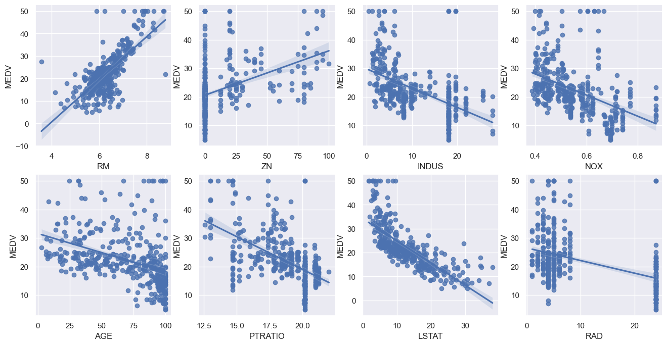
regplot 구하기
fig,axs = plt.subplots(figsize=(16,8), ncols=4,nrows=2)
lm_features = ['RM','ZN','INDUS','NOX','AGE','PTRATIO','LSTAT','RAD']
for i, feature in enumerate(lm_features):
    row = i//4
    col = i%4
    sns.regplot(x=feature,y='MEDV',data = boston_data, ax = axs[row][col])
plt.show()
out:
선형회귀
y = boston_data['MEDV']
X = boston_data.drop(['MEDV'],axis=1,inplace=False)

X_train,X_test,y_train,y_test = train_test_split(X,y,test_size=0.3,random_state=42)

lr = LinearRegression()
lr.fit(X_train,y_train)
y_pred = lr.predict(X_test)
mse = mean_squared_error(y_test,y_pred)
rmse = np.sqrt(mse)
print('MSE : {0:.3f}, RMSE : {1:.3f}'.format(mse,rmse))
print('Variance Score : {0:.3f}'.format(r2_score(y_test,y_pred)))

print("절편값: ",lr.intercept_)
print("회귀 계수 값: ", lr.coef_)
out:
MSE : 28.871, RMSE : 5.373
Variance Score : 0.691
절편값:  32.9932233550285
회귀 계수 값:  [-1.12990963e-01  4.49594371e-02  5.75447722e-02  1.18099414e+00
 -1.72522169e+01  4.27138350e+00 -1.99977624e-02 -1.40633199e+00
  2.77671705e-01 -1.68192666e-02 -8.96637094e-01  9.07231436e-03
 -3.64600546e-01]
fold validation
coeff = pd.Series(data = np.round(lr.coef_,1), index = X.columns)
print(coeff.sort_values(ascending=False))

neg_mse_scores = cross_val_score(lr,X,y,scoring='neg_mean_squared_error', cv=5) ## 여기만 negative를 선언했다.
rmse_scores = np.sqrt(-1*neg_mse_scores)
avg_rmse = np.mean(rmse_scores)
print('5 folds each negative Mse scores: ',np.round(neg_mse_scores,2))
print('5 folds each RMSE scores: ',np.round(rmse_scores,2))
print('5 folds each avg RMSE: {0:.3f}'.format(avg_rmse))
out:
RM          4.3
CHAS        1.2
RAD         0.3
INDUS       0.1
ZN          0.0
AGE        -0.0
TAX        -0.0
B           0.0
CRIM       -0.1
LSTAT      -0.4
PTRATIO    -0.9
DIS        -1.4
NOX       -17.3
dtype: float64
5 folds each negative Mse scores:  [-10.64 -19.6  -32.05 -65.53 -27.51]
5 folds each RMSE scores:  [3.26 4.43 5.66 8.09 5.24]
5 folds each avg RMSE: 5.338
gpt로 다시 배우는 개발