개요
딥러닝이 이미지나 텍스트와같은 비구조화된 데이터에만 사용되는 것 뿐만 아니라 구조화된 데이터에서도 지속적으로 시도를 하고 있다. 이번에 소개할 예제는 이러한 데이터를 다루기 위한 Keras만의 전처리 방식에 대해 소개할 예정이다. 해당 내용은 Keras의 창시자라 불리는 프랑수아 숄레가 작성했으며 해당 내용은 여기에 있다.
데이터셋 소개
이번에 분석할 데이터셋은 Cleveland Clinic Foundations for Heart Disease에서 제공한 데이터셋으로 나이, 성별, 기저질환등으로 심장병 유무를 예측하기 위해 만들어졌다. 각각의 변수는 다음과 같다.
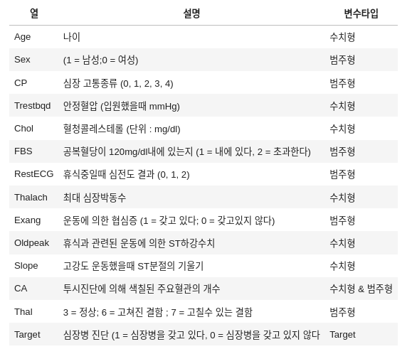
구조화된 데이터같은 경우 전처리하기 전에 선행되어야 할 것은 해당 변수에 대한 타입을 파악하는 것이다. 그렇기에 해당 변수 타입을 먼저 고려한 다음 전처리가 이루어져야 한다.
데이터 준비하기
import tensorflow as tf
# tensorflow 2.6.0이상
import numpy as np
import pandas as pd
from tensorflow import keras
from tensorflow.keras import layers

file_url = "http://storage.googleapis.com/download.tensorflow.org/data/heart.csv"
dataframe = pd.read_csv(file_url)

dataframe.shape
#(303, 14)

dataframe.head()
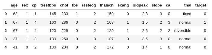
해당 데이터프레임은 다음과 같이 이루어져 있는걸 확인할 수 있다.
데이터프레임을 train, validation set으로 나누고 keras에서 사용할 수 있는 데이터셋으로 변환하기
val_dataframe = dataframe.sample(frac=0.2, random_state = 1337)
train_dataframe = dataframe.drop(val_dataframe.index)

def dataframe_to_dataset(dataframe):
    dataframe = dataframe.copy()
    labels = dataframe.pop('target')
    ds = tf.data.Dataset.from_tensor_slices((dict(dataframe), labels))
    ds = ds.shuffle(buffer_size = len(dataframe))
    ds = ds.batch(32)
    return ds

train_ds = dataframe_to_dataset(train_dataframe)
val_ds = dataframe_to_dataset(val_dataframe)
우선 데이터프레임에서 train set과 validation set으로 나누기 위해 pd.DataFrame.sample을 이용해 데이터셋에 20%정도를 샘플링해 validation set으로 만들고 나머지를 train set으로 지정한다.
그 다음
- 데이터프레임을 깊은 복사를 하고(
dataframe = dataframe.copy()) - labels를 target에서 뽑아낸다.(
labels = dataframe.pop('target')) - 이후 tf.data.Dataset.from_tensor_slice를 이용해 labels이 빠진 dataframe의 딕셔너리형태를 x로 두고 labels를 y로 두어 데이터프레임을 keras에서 사용할 수 있는 데이터셋으로 변환한다. (
ds = tf.data.Dataset.from_tensor_slices((dict(dataframe, labels))) - 데이터셋에 랜덤성을 더하기 위해 섞여준다. (
ds = ds.shuffle(buffer_size = len(dataframe))) - 마지막으로 배치사이즈(32)에 맞게 자르면 완성된다. (
ds = ds.batch(32))
Keras layer를 활용해 전처리하기
우리는 앞서서 변수에 대한 타입을 미리 확인했으며 해당 데이터셋의 변수는 크게 3가지로 분류할 수 있다.
-
범주형 변수
볌주형 변수에 속하는 변수는sex,cp,fbs,restecg,exang,ca,thal이 있다. 이 중에서thal을 제외한 다른 변수들은 정수로 범주가 결정되어 있다.
Keras에서는 정수로 되어 있는 범주형 변수를 다루는 Tool은CategoricalEncoding()과IntegerLookup()이 있다. 둘의 차이는 다음과 같다. 이번 예제같은 경우 추론할때 입력값의 범위가 벗어날 수 있기 때문에IntegerLookup()을 사용한다.CategoricalEncoding()은 input의 범위를 알아야 하고 범위를 벗어나면 에러가 발생한다.IntegerLookup()은 input에 대한 룩업 테이블을 만들고 모르는 Input에 대한 출력값은 보존된다.
-
문자열로 이루어진 범주형 변수
한편thal과 같이 문자열로 범주를 결정하는 변수는StringLookup()을 사용해 one-hot 인코딩을 한다.
-
수치형 변수
age,trestbps,chol,thalach,oldpeak,slope는 수치형 변수에 속하고 이러한 변수들은Normalization()을 이용해 정규화한다.
우리는 이러한 작업을 하기 위해 2가지 유틸리티 함수를 정의할 것이다.
from tensorflow.keras.layers import IntegerLookup, Normalization, StringLookup

def encode_numerical_feature(feature, name, dataset):
    # 변수들에 정규화층(Normalization layer)을 생성한다.
    normalizer = Normalization()

    # 변수들을 생성하는 데이터셋을 구축한다.
    feature_ds = dataset.map(lambda x, y : x[name]) #(None,)
    feature_ds = feature_ds.map(lambda x : tf.expand_dims(x, -1)) #(None, 1)

    # 데이터를 정규화한다.
    normalizer.adapt(feature_ds)

    # 정규화한 데이터를 원래 feature에 적용한다.
    encoded_feature = normalizer(feature)
    return encoded_feature #(None, 1)

def encode_categorical_feature(feature, name, dataset, is_string):
    lookup_class = StringLookup if is_string else IntegerLookup
    # 문자열를 수치형 인덱스로 변하는 룩업층을 생성한다.
    lookup = lookup_class(output_mode = 'binary')

    # 변수들을 생성하는 데이터셋을 구축한다.
    feature_ds = dataset.map(lambda x, y : x[name])
    feature_ds = feature_ds.map(lambda x : tf.expand_dims(x, -1))

    # 가능한 문자열들의 집합을 학습시키고 이러한 것들을 고정된 수치형 인덱스로 부여한다.
    lookup.adapt(feature_ds)

    # 문자열 입력값을 수치형 입력값으로 바꾼다.
    encoded_feature = lookup(feature)
    return encoded_feature
우선 encode_numerical_feature부터 먼저 살펴보자.
- 정규화 Layer를 먼저 정의한다. (
normalizer = Normalization()) - 데이터셋 내에 있는 feature를 하나 가져온다 (
feature_ds = dataset.map(lambda x, y : x[name])) - Feature에 차원을 1개 추가한다. (
feature_ds = feature_ds.map(lambda x : tf.exapnd_dims(x, -1))) - feature_ds에 정규화를 적용한다. (
normalizer.adapt(feature_ds)) - 미리 정의한 Keras Input layer에 값을 적용한다. (
encoded_feature = normalizer(feature))
encode_categorical_feature()는 다음과 같은 과정을 거친다.
- string이면 StringLookup을 사용하고 그렇지 않으면 IntegerLookup을 사용한다. (
lookup_class = StringLookup if is_string else IntegerLookup) - 우리가 할 task는 이진분류이기 때문에 lookup class에 output_mode를
binary로 설정한다. (lookup = lookup_class(output_mode = 'binary') encode_numerical_feature2번 3번과 동일``- feature_ds에 룩업테이블을 학습시킴 (
lookup.adapt(feature_ds)) - 미리 정의한 Keras Input layer에 값을 적용시킨다.(
encoded_feature = lookup(feature))
모델 설계하기
# 정수형 변수에서 인코딩된 범주형 변수들
sex = keras.Input(shape=(1,), name = 'sex', dtype = 'int64')
cp = keras.Input(shape=(1,), name = 'cp', dtype = 'int64')
fbs = keras.Input(shape=(1,), name = 'fbs', dtype = 'int64')
restecg = keras.Input(shape=(1,), name = 'restecg', dtype = 'int64')
exang = keras.Input(shape=(1,), name = 'exang', dtype = 'int64')
ca = keras.Input(shape=(1,), name = 'ca', dtype = 'int64')

# 문자열 변수에서 인코딩된 범주형 변수
thal = keras.Input(shape=(1,), name="thal", dtype="string")

# 수치형 변수
age = keras.Input(shape=(1,), name="age")
trestbps = keras.Input(shape=(1,), name="trestbps")
chol = keras.Input(shape=(1,), name="chol")
thalach = keras.Input(shape=(1,), name="thalach")
oldpeak = keras.Input(shape=(1,), name="oldpeak")
slope = keras.Input(shape=(1,), name="slope")

all_inputs = [
    sex,
    cp,
    fbs,
    restecg,
    exang,
    ca,
    thal,
    age,
    trestbps,
    chol,
    thalach,
    oldpeak,
    slope,
]

# 정수형 범주 변수들
sex_encoded = encode_categorical_feature(sex, "sex", train_ds, False)
cp_encoded = encode_categorical_feature(cp, "cp", train_ds, False)
fbs_encoded = encode_categorical_feature(fbs, "fbs", train_ds, False)
restecg_encoded = encode_categorical_feature(restecg, "restecg", train_ds, False)
exang_encoded = encode_categorical_feature(exang, "exang", train_ds, False)
ca_encoded = encode_categorical_feature(ca, "ca", train_ds, False)

# 문자열 범주 변수
thal_encoded = encode_categorical_feature(thal, "thal", train_ds, True)

# 수치형 변수
age_encoded = encode_numerical_feature(age, "age", train_ds)
trestbps_encoded = encode_numerical_feature(trestbps, "trestbps", train_ds)
chol_encoded = encode_numerical_feature(chol, "chol", train_ds)
thalach_encoded = encode_numerical_feature(thalach, "thalach", train_ds)
oldpeak_encoded = encode_numerical_feature(oldpeak, "oldpeak", train_ds)
slope_encoded = encode_numerical_feature(slope, "slope", train_ds)
우선 input을 정의하고 위에 정의한 함수를 바탕으로 인코딩한다.
all_features = layers.concatenate(
[
sex_encoded,
cp_encoded,
fbs_encoded,
restecg_encoded,
exang_encoded,
slope_encoded,
ca_encoded,
thal_encoded,
age_encoded,
trestbps_encoded,
chol_encoded,
thalach_encoded,
oldpeak_encoded,
]
)
x = layers.Dense(32, activation="relu")(all_features)
x = layers.Dropout(0.5)(x)
output = layers.Dense(1, activation="sigmoid")(x)
model = keras.Model(all_inputs, output)
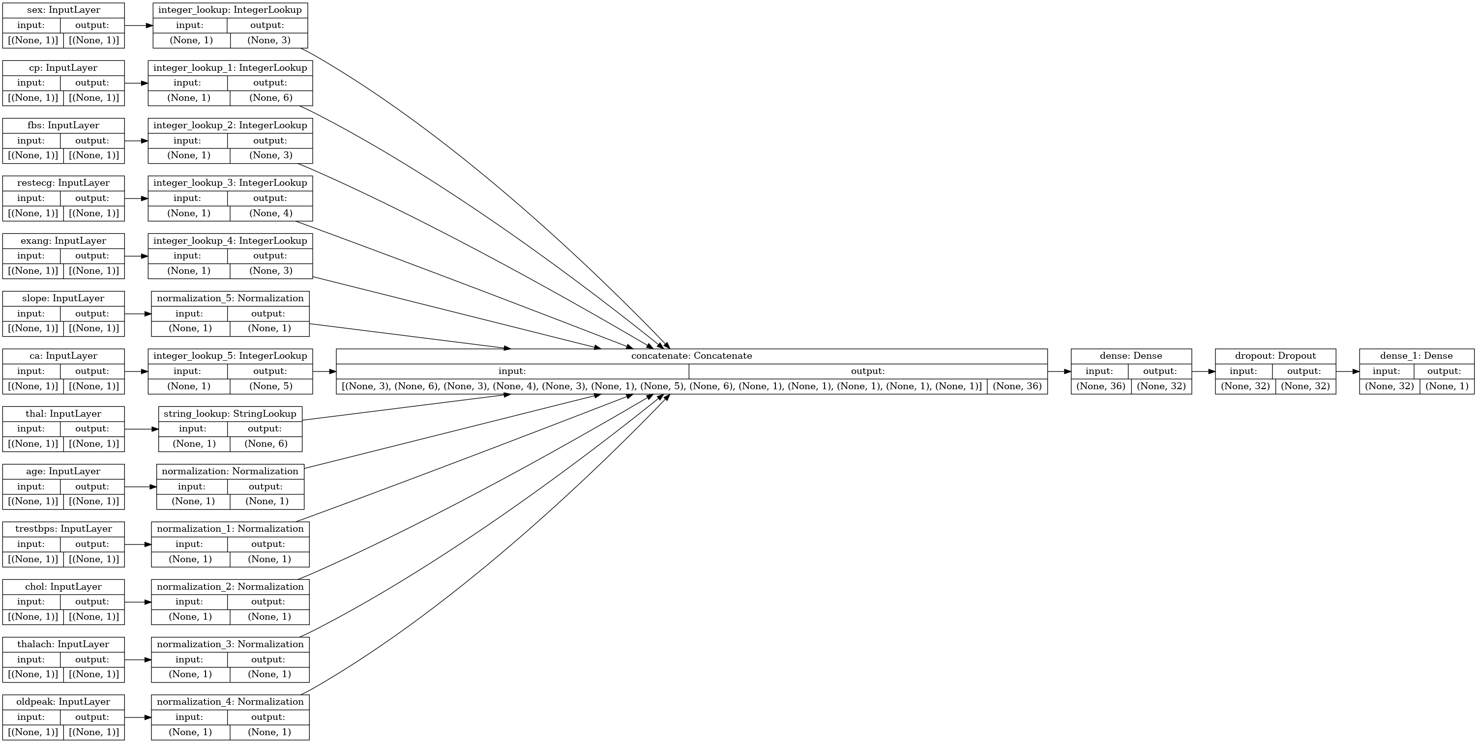
model.compile("adam", "binary_crossentropy", metrics=["accuracy"]) 그 다음 인코딩한 함수들을 전부 concat한 이후 Fully-connected layer를 거치고 ReLU함수로 activation한다. Dropout을 거친 다음 Fully-connected layer를 거친다음 Sigmoid함수로 이진분류를 한다. 해당 모델의 loss는 binary crossentropy loss를 사용하고 optimizer는 Adam을 사용할 것이다.
이를 그림으로 표현하면 다음과 같다.
모델 훈련 & 추론
model.fit(train_ds, epochs=50, validation_data=val_ds)해당 모델을 50 Epoch정도 학습시키고 validation data를 사용해 정확도를 측정한다.
sample = {
    "age": 60,
    "sex": 1,
    "cp": 1,
    "trestbps": 145,
    "chol": 233,
    "fbs": 1,
    "restecg": 2,
    "thalach": 150,
    "exang": 0,
    "oldpeak": 2.3,
    "slope": 3,
    "ca": 0,
    "thal": "fixed",
}

input_dict = {name: tf.convert_to_tensor([value]) for name, value in sample.items()}
predictions = model.predict(input_dict)

print(
    f'우리의 모델에 의하면 이 환자는 {100* predictions[0][0]}%확률로 심장병을 갖고 있다.')
추론을 할 경우 sample dictionary data를 만들고 해당 dictionary를 tensorflow에 맞게 Tensor로 변환한다. 그리고 model.predict를 활용해 예측한다.
회고
외적인 면에서 힘들었던 점은 구조화된 데이터같은 경우 tensorflow 2.6.0 이상에서만 사용할 수 있다. 2.6.0같은 경우 cudatoolkit이 필요하므로 기존과 다르게 설치단계에서 몇단계를 거쳐야 gpu연산이 가능해진다. 여기에서 생각보다 시간이 꽤 걸렸다.
내용적인 면에서는 Keras 작동방식을 조금 더 이해할 수 있었다. 코드 한줄한줄 분석하고 찾아내는 과정에서 코드를 보는 시야가 조금 더 넓어졌다는 생각이 들었다.